High crest factor signals, such as CDMA/WCDMA, may have PAPR (Peak-to-Average Power Ratio) as high as 10dB. To ensure the most accurate power measurement, the average power of the signal should not exceed +20dBm. For example the peak power of the signal should not exceed +30dBm if its PAPR is 10dB.
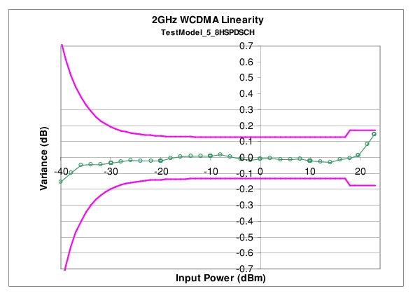
A MA241xxA series sensor’s linearity graph of a WCDMA (TestModel_5_8HSPDSCH) signal with 10 dB PAPR is shown below:
Sensor Linearity Graph
Multitone Signals
The sensor is a True-RMS sensor that can measure very wide bandwidth modulation without much restriction. The only limitation is the frequency flatness of the sensor. Because the sensor’s sensitivity is not identical for all frequencies and when measuring multitone signals, the frequency entered into the sensor’s application should be the average frequency of all significant tones. The sensor has an additional uncertainty of 0.05 dB for every 1 GHz tone separation when measuring multitone signals.
For example, a dual tone signal of 2 GHz and 4 GHz may have an additional measurement error of 0.1 dB (0.05 dB × 2) when the application frequency is set to 3 GHz.
Advanced Features / Enhanced Modulation
Enhanced Modulation is available with the MA242x8A sensors only. Enhanced modulation can be enabled under Tools/Advanced Features menu. It is recommended to measure pulse modulated signal with period shorter than 30 µs and crest factor up to 10 dB. The user can also examine the signal in Scope mode set to one sample per point with and without Enhanced modulation, and choose the setting that yields a better defined waveform.
The enhanced modulation has a different algorithm to compute the final power reading based on sampled voltages, and is available in all the modes supported. The crossover power between ranges are set 3 dB lower in enhanced modulation to allow for the modulated signal.
When measuring the average power of a time varying or modulated signal with a modulation bandwidth (BW) which is much greater than the signal channel of the sensor, averaging of the power is performed in the sensor hardware (detectors and or preamplifiers). For the case of the MA24x08A, MA24x18A and MA24126A; the signal channel BW is 50 kHz. Signals modulated at MHz rates will be averaged in the hardware and no special considerations are required.
When measuring signals with modulation frequency components near, or below, the signal channel bandwidth, average power readings may be seen to fluctuate over time. This fluctuation may be reduced through careful selection of the aperture time and averaging number. Ideally, the aperture time should be chosen to be an integer multiple of the modulation frequency. If this can be done, then the average power reading will be stable for each measurement update. For modulations with multiple frequencies present, or with significant modulation components with periods longer than the maximum aperture time (300 ms for MA24108A, MA24118A, MA24126A and 1 s for MA242x8A), averaging will have to be increased to obtain a stable reading. If the measurement update rate is very close to the period of the modulation, a low frequency “beat note” can result. If the frequencies are very close, the beat note can be very low in frequency, and therefore require very long averaging times to remove. In this case it is suggested that the aperture time be changed to result in a higher frequency beat which is easier to average out.
Settling Time
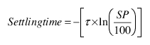
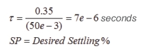
The signal channel bandwidth of the MA241xxA series and MA242x8A series power sensor supports a rise time of about 8 µs. The ADC sample period is approximately 7.6 µs. Thus it will take more than one ADC sample for the signal channel hardware to completely settle in response to a step change in input power. The hardware settling time for the MA241xxA series power sensor can be estimated by assuming a single pole response with 50 kHz bandwidth:
where:
For small settling percentages, it is quite likely that the noise per ADC sample will be larger than the desired settling percentage, thus averaging or decimation of ADC samples will have to be used to reduce the noise. Averaging will, of course, increase the settling time of the measurement in direct proportion to the averaging number used.
It is important to note that the settling time described above strictly applies only to increasing power steps (rise time). Settling to decreasing power steps is typically slower. For settling decreasing power steps to 1 % or 0.1 %, the settling will typically be within a factor of 2 or 3 of the calculation above. Settling to 0.01 % or less may take considerably longer.
Noise and Time Resolution in Scope Mode
In Scope mode (and in all other modes), the MA24x08A, MA24x18A and MA24126A is sampling at full speed, which is approximately once every 7 µs. When the period chosen for Scope mode exceeds the number of data points times this period, then multiple ADC samples are averaged to form each data point. Therefore there is a trade-off between time resolution (many data points) and trace noise. To minimize trace noise, choose less data points. Of course for recurrent waveforms, trace averaging can always be used to reduce trace noise if a large number of points is desired. This would however tend to increase the over-all measurement time.
Optimizing Internal Triggering
Sometimes it can be difficult to obtain consistent triggering in scope or Time Slot mode. Here are some points to consider when choosing triggering parameters:
• It is more difficult to trigger on signals which are slowly varying with time. Noise in the signal channel can result in false triggers. In this case, try setting the trigger level at powers away from the bottoms of the measurement ranges. The trigger crossover power for the MA24105A, MA24106A, MA24108A, MA24118A, and MA24126A is about +2 dBm. Thus it can be advantageous to avoid setting the trigger at powers just above +2 dBm, and powers just above –20 dBm where the trigger signal is noisy. The trigger crossover power for the MA24208A and MA24218A is about +4 dBm. Thus it can be advantageous to avoid setting the trigger at powers just above +4 dBm, and powers just above –16 dBm where the trigger signal is noisy.
• Modulated signals can appear “noisy” and also result in false triggers. In this case, adjusting the trigger level may not help. Sometimes there may be a portion of the signal with less modulation, or less “noise-like” modulation which can be triggered on with more success. Try using a different trigger point and adjusting the trigger delay to shift the waveform in time to see the desired section.
• False triggers due to either noise or noise-like modulation can be reduced by increasing the trigger noise immunity parameter for the MA24108A, MA24118A, and MA24126A and invoking hysteresis for the MA242x8A. Using noise immunity will result in a slight positive trigger delay, but this can be made up for by introducing a negative trigger delay with the trigger delay parameter.
• The trigger settings should always be optimized before trace averaging is applied. If trace averaging is used when the trigger is not stabilized, the displayed waveform will not be an accurate representation of the signal. First optimize the trigger, then apply trace averaging.
Noise Floor in Scope Mode
The noise level or “floor” displayed in scope or Time Slot mode in PowerXpert when using low averaging may seem to be higher than what would be expected. This is due to the way noise is dealt with when converting power into dBm for display. With no input power, the values of the ADC samples vary about some value which corresponds to zero power. Ideally there are equal number of samples above and below this value. The samples which are below this value correspond to “negative” power. This is non-physical, and does not truly mean there is negative power flow to the sensor, it is simply a by product of noise in the signal channel. If these samples are displayed in linear power units such as mW, then the noise floor will be as expected. However there is a problem when converting to logarithmic units such as dB. Because taking the logarithm of negative numbers is not generally allowed, the absolute value of the samples is usually taken before taking the logarithm. This has the drawback of increasing the average value of the samples, artificially increasing the apparent noise floor. When the averaging is increased, the noise floor will go down. The apparent noise floor can be estimated using:
NF = 0.8 x noise
where:
NF = the average linear power or noise floor due to taking absolute value of power samples
noise = the noise power in linear units on a 1 sigma basis