LRL (Line-Reflect-Line) uses two (or more) transmission lines and a reflect standard (for each port). The line lengths are important as it is required that the two lines look electrically distinct at all times (meaning it will not work at DC nor at a frequency where the difference in length is an integral number of half wavelengths). The reflect standard is assumed to be symmetric and without a high return loss. The lines are assumed perfect (no mismatch), and are usually airlines for coaxial calibrations, although other structures can be used. On-wafer transmission lines can be very good and this calibration approach will work well if the required probe movement can be managed.

LRM (Line-Reflect-Match) and ALRM (Advanced Line-Reflect-Match) calibrations have one of the lines above replaced with a match (or load). The load is modeled/characterized (or assumed perfect). Since only one line is involved, this calibration can work down to DC and up to very high frequencies (practically limited by the match knowledge/characterization). Variations allow one of the match measurements to be traded for a pair of additional reflect measurements (a second reflect standard is needed). Because of the requirement that the reflect standards be distinct, the calibration may become band limited.

In the limiting case of a match that is assumed perfect, or at least assumed symmetric, this calibration reduces to the classical LRM. The added flexibility is in the ability to define asymmetric load models and to use multiple reflect standards as discussed above. The double reflect methodology allows one to feed into a load modeling utility where the load model can be further optimized.

Some parameters to keep in mind:

In addition to the LRL frequency limits, the line length is used for some reference plane tasks. The fundamental reference plane of an LRL/ALRM calibration is in the middle of the first line. If the reference plane is required at the ends of this line, the line length (and loss which can also be entered) is used to rotate the reference planes to the desired location. The line length delta is also used for some root choice tasks, although the accuracy required on this entry is less. It is allowed to enter a 0 length for line 1 even when the length is physically non-zero as another way of forcing the reference planes to the middle. There are some caveats:

As mentioned above, the usable frequency range for LRL is set by the line length delta. Strictly speaking, the electrical length should be between 0 and 180 degrees for all frequencies of interest although some margin is usually desired to account for line parasitics, spurious mode launches and other problems. In general, the delta should be kept between 10 and 170 degrees or 20 and 160 degrees. Practically speaking, one can usually be more aggressive on the lower number and will want to be less aggressive on the upper number:

Where ΔL is in meters, vph is the phase velocity of the line (= 2.9978 108m/s = c for air dielectric) and f can be any frequency in the range of interest, expressed in Hz.

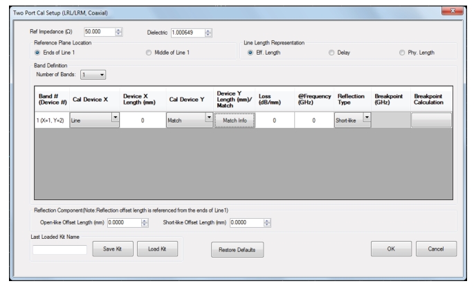
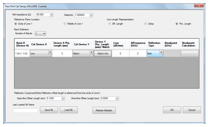
If this range is too small for the application, multiple lines and multiple bands can be used which will be discussed shortly. The single-band version of the dialog is highlighted in Figure: TWO PORT CAL SETUP (LRL/LRM, COAXIAL) Dialog Box. Two devices must be defined and the first (Cal Device X) must be a line which has a length associated with it in millimeters (air equivalent) or in picoseconds of delay. Note that the Cal Device X in the first band has an added role when the reference plane choice ‘Ends of Line 1’ is selected. The length of this Cal Device X will be rotated out from the final error coefficients to place the reference planes at its ends. The basic LRL/LRM/ALRM algorithm places the reference plane in the middle.

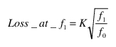
A loss and frequency dependence for the line can be optionally specified (loss defaults to 0 dB). The loss is in per-unit-length terms and can be assumed flat with frequency by entering 0 in the frequency field. If a non-zero value is entered, the loss value entered is assumed to be at that frequency and a square-root-of-f scaling will be used at other frequencies. In other words, if the loss K is entered at frequency f0 then the value at frequency f1 will be computed as:

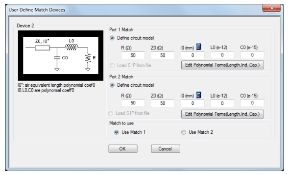
The second device (Cal Device Y) can either be another line or a match. If another line, its length/delay should be entered although this value will be primarily used to help with root choice. The loss values for Cal Device X will be used for Cal Device Y. If the second device is a match, the model for that match may be entered using the sub-dialog (assumed infinite return loss by default). As discussed previously, if both reflects are selected and a match is being used for Cal Device Y, then the ALRM algorithm will be used. The entered load model is only then used for the first part of the calculation to help the optimizer more quickly generate a better fit for the simplified match model. Also, only one of the match measurements is needed for this algorithmic variant and the match to be used is selected in the sub-dialog.

Because of the phase restrictions discussed above, each LRL calibration is fundamentally band-limited to something on the order of an 8:1 to 17:1 frequency range (and some users may restrict it further for measurements requiring very low uncertainties when the line losses are low). To cover wider frequency ranges and to, for example, use LRM/ALRM for part of the frequency range, the concept of Multiband LRL was generated. Various combinations of standards (staying within the LRL/LRM/ALRM family) can be used to cover multiple bands and hence cover the extended range. The concept of the ‘breakpoint frequency’ is needed that defines when the calibration coefficients are taken from the lower band measurements and when they are taken from the upper band measurements. This process does not affect how the measurements are done. It just changes which data (from an over-determined set) is used to compute the calibration coefficients. The calibration process is optimized so that if a particular standard is used in multiple bands, it only needs to be measured once.

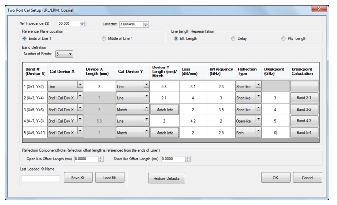
The setup dialog is shown in Figure: TWO PORT CAL SETUP (LRL/LRM, COAXIAL) Dialog Box with the maximum of 5 allowed bands selected. In some sense, each band is a new LRL/LRM/ALRM calibration covering some subset of the desired frequency range. All of the bands share the same open-like and short-like reflects although one can choose between those two independently in each band (or use both for ALRM in any band). In each band, one must choose two lines or one line and a match and those devices can be shared amongst the bands. As an example, it is not unusual to share one line in all of the bands and then the 2nd line in each band is chosen to create an ever-decreasing ΔL as the band number increases (thus each subsequent band is to be used in a higher frequency sub-range). In the higher numbered bands, any devices in the previous bands can be used. Note that loss entries are local to a band in order to allow the user to correct for deviations from the square-root-of-f loss frequency dependence model.

To illustrate a multi-band setup, we will work through a design example where the calibration range is to be 200 MHz to 70 GHz and we wish to not exceed 20 to 160 degree relationships and do the calibration with only LRL using air dielectric lines. Since the high-to-low ratio is less than 83 the calibration can be accomplished in 3 bands under these conditions. It is desired to use a common line of length 10 cm for all bands.

If the first band must work down to 200 MHz with a 20 degree ΔL limit, then the first ΔL=8.333 cm so the second line should be 18.333 cm long. This first band, using the 160 degree limit, should be able to reach 1.6 GHz. To allow some band overlap (and improve uncertainties a bit more), we will choose the 20 degree lower limit of the second band to be a bit lower than 1.6 GHz and select 1.4 GHz. This implies a second ΔL of 1.19 cm. Since we wish to re-use the 10 cm line in this band, the second line in the second band should be 11.19 cm long with a 160 degree-based frequency limit of 11.2 GHz. For the third band, we will again aim for a value under the previous band’s 160 degree limit and select 10 GHz. This leads to a third ΔL of 1.67mm or a final line length of 10.167 cm.

Summarizing:

In this full calibration example, there are a total of four lines to be measured (along with whatever reflect standard(s) was (were) selected). Although not all of the frequency range data for each device will be used (e.g., band 2 Cal Device Y data for frequencies below 1.497 GHz or above 10.58 GHz will not be used), all devices will be swept over the whole calibration frequency range in order to simplify sweep control and minimize overhead.

Here the breakpoints were calculated off-line using the geometric mean of the upper limit of the lower band and the lower limit of the upper band. The recommended values that would be generated by the instrument would be different since it uses the 10 to 160 degree process instead of the 20 to 160 degree limit we selected for this example. These slight shifts in breakpoint will generally have limited effect of the results (<0.03 dB error generally at the breakpoint in this case) but if one gets more aggressive with the angle limits, errors can increase. This is less true if the lines are lossy (as in a PC board environment) than if the losses are very low.

 

The Cal Merge (concatenation) utility can also be used with any other calibration types in order to cover a wider frequency range.

Some information is requested about the reflection although a full characterization is not needed. The information is used in some root-choice activities and it only needs to be known if the reflect behaves more like an open or a short (since typically opens and shorts are used as the reflect standard). The offset length is used to dynamically move the reference planes around so the algorithm will know what the reflect looks like at any given frequency. Normally, the reflection offsets are always entered relative to the ends of line 1 (even if a different final reference plane is selected). If a non-zero length line 1 is used but 0 is entered for the length (another approach to get reference planes in the middle), the reflection offsets must still be relative to the ends of the physical line 1, so the offset entries may be negative in this case.

In the double reflect ALRM methodology it is important that the reflect standards be distinct. More specifically, they must be distinct when rotated to the reference plane at the center of line 1. Since large offset lengths will lead to many more degeneracies, this double reflect option will generally be used when offset lengths are smaller (such as in on-wafer of fixtured calibrations).

When a single reflect approach is taken within ALRM, it behaves like a classical LRM. For slightly more advanced use, complete load models can be entered for the two matches independently. The same model as described for SOLT applies.

At the highest level, two reflects are measured per port to allow more optimized information to be obtained. When the double reflect methodology is selected, an optimization routine can be selected which can lead to a load model.

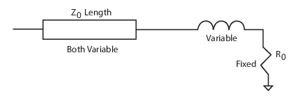
The structure in Figure: Load Model/Characterization for ALRM below is used (similar to that for the general model except no capacitance). The resistance element is assumed known (whether from DC measurements or other parametric data). The inductance and transmission line parameters can be optimized over given ranges.

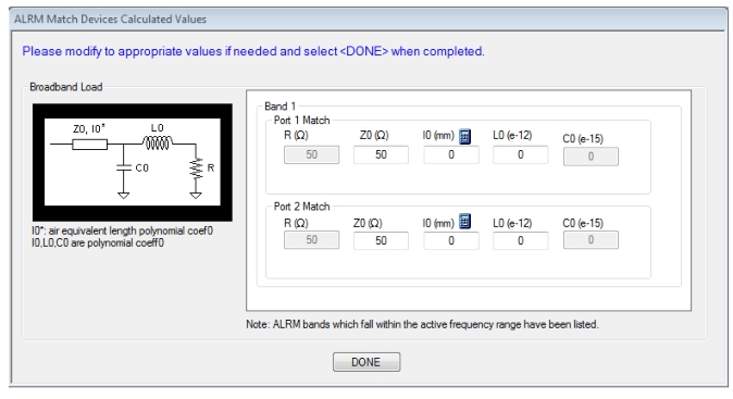
The dialog box shown in Figure: ALRM MATCH DEVICES CALCULATED VALUES Dialog Box (BAND 1) below pertaining to this model will appear after the main calibration steps are complete. At that point, the fit model can be used (default) or modified values can be entered. A model will be suggested by the algorithm but can be overridden in this dialog.

The dialog boxes shown above are for coaxial or non-dispersive line types. For waveguides and microstrips, the only change is the addition of items at the top of the dialog to specify the media (see Figure: An Example LRL/ALRM Setup Dialog for a Waveguide Line Type and Figure: An Example LRL/ALRM Setup Dialog for a Microstrip Line Type below).

An example LRL/ALRM setup dialog for a waveguide line type is shown in Figure: An Example LRL/ALRM Setup Dialog for a Waveguide Line Type. Note the cutoff and dielectric constant line items that are added.

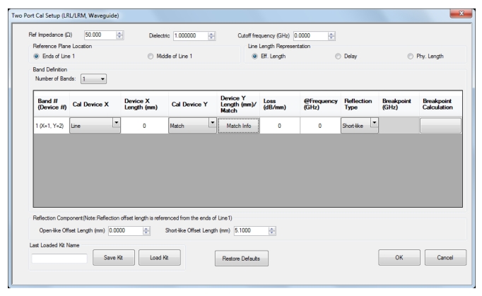
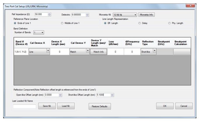
An example LRL/ALRM setup dialog for a microstrip line type is shown Figure: An Example LRL/ALRM Setup Dialog for a Microstrip Line Type. Note the media line items that have been added (the microstrip info sub-dialog is described earlier).

When using the double-reflect ALRM method, it is important to note that the reflections must produce distinct reflection coefficients when rotated to the central reference plane. When the reflect offset lengths start to become large, this gets to be more difficult over large frequency ranges. In an on-wafer environment when the offset lengths are typically very short, this does not present a problem but it can be an issue in coax. Since the load modeling is most commonly an issue in high frequency on-wafer measurements, this behavior is usually consistent with the applications.