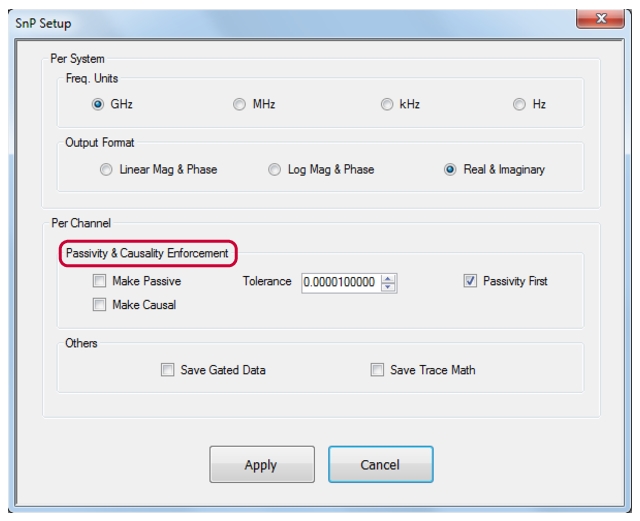
When S-parameter data from network extraction or just from measurement are used in external simulators, there are sometimes requirements on the data in terms of passivity or causality for simulation convergence or for other performance requirements. It is possible to enforce these characteristics on .sNp saved data (either measurement or network extraction) although changes are made to the data in that process. This section will discuss the enforcement procedures and some of the implications. Figure: SnP Setup Dialog shows the sNp setup dialog for enforcing Passivity and Causality, which can be accessed via:

Main | System | Setup | Misc Setup | SnP Files Setup | SNP SETUP dialog

Here, this is defined as the 2-norm of the S-parameter matrix being less than or equal to one. This is equivalent to the eigenvalues of the S-parameter matrix all being less than or equal to one in magnitude. The reader may associate passivity with |S21| ≤1 but that is not a sufficient requirement for most situations where convergence is an issue.

In practice, many passivity violations (on actually passive devices; those not capable of energy conversion) arise from calibration problems (standards issues), cable or drift issues, or repeatability variances (connections or probe touchdowns). Ideally, those issues should be addressed to improve the basic data quality. However, for very low loss devices/fixtures, the data may only be marginally non-passive and it may be expedient to coerce that data to proceed with a simulation, system design, etc. The Make Passive selection will do this on all .sNp saves but it is up to the user to assess if the changes being made to the data are acceptable.

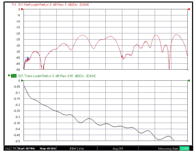
Typically the changes are quite small if the calibration quality is good. As an example, the measurement of an adapter chain is shown in Figure: Measurement of an Adapter Chain and an Enforced-passivity Version of that Data and the passivity-enforced result is overlaid on top (aside: as stated elsewhere, this can be done by placing the instrument in Hold and recalling the .s2p file that was saved (with passivity enforcement in this case); the actual measured data was saved to trace memory). One can see some slight changes under 2 GHz where the insertion loss is the lowest. The ‘enforced’ insertion loss at very low frequencies is increased by ~0.005 dB and the return loss is increased by about 1 dB at the –40 dB level. This level of change is far below the uncertainty levels and is likely to be acceptable.

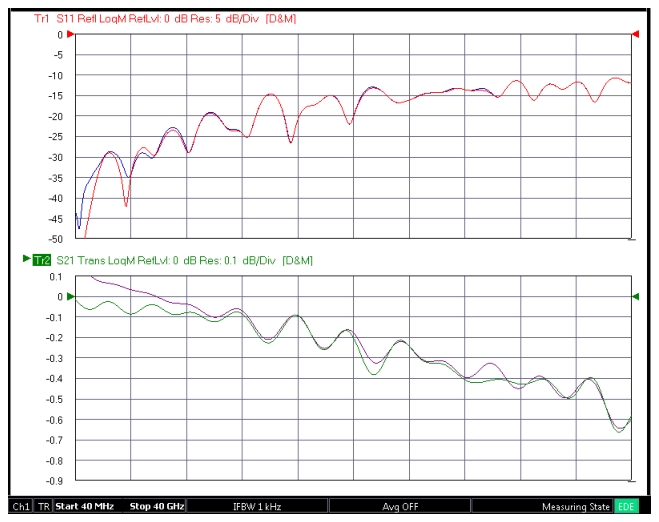
If the calibration quality is poor, the changes can be more dramatic. To simulate this, a non-existent transmission line was de-embedded from the original calibration so insertion loss reads artificially low (and indeed shows insertion gain for the adapter chain at low frequency). The change from passivity enforcement in this case exceeds 0.1 dB at low frequencies and is noticeable at higher frequencies (see Figure: Passivity Enforcement with Calibration Problems). This happens because the introduced calibration degradation also caused apparent mismatch levels to be much higher. This is important since now the 2-norm can exceed unity even if |S21| is ~-0.4 dB. The changes made in enforcement here are significant and, if they occurred with a real calibration, one might want to investigate the calibration and measurement (cables, connectors, standards, etc.) before continuing with the enforced data.

The passivity enforcement works by re-scaling the eigenvalues of the S-parameter matrix in a self-consistent way and then regenerating the S-parameters from the new eigenvalues. The consistency of this approach is important since one wants to maintain the relationship between reflection and transmission parameters as much as possible to lessen the effect on any other system calculations.

The user is given some control over how much less than unity the 2-norm must be since some simulators screen for passivity using tests that are more-or-less stringent. A ‘tolerance’ variable is provided and if the entry is x, the maximum eigenvalue magnitude will be 1-sqrt(x). The default value for x is 0.00001 and is allowed to go as high as 0.001 for the more stringent tests.

Causality is the state of not being dependent on the given parameter value at an earlier point in time. This has a number of implications:

As with passivity, this condition may be required of S-parameter data that is to be used in certain simulations and, again, there is a way to coerce data to make this happen. In practice, causality violations can occur from calibration and drift issues (particularly nonlinear phase drift) and from measurements of very broadband devices with a small measurement bandwidth (so there is little roll-off). This last statement follows from the observation that any limited bandwidth set of data, when transformed to the time domain, will have energy for t<0. This energy becomes significant if there is little parameter roll-off at the highest measurement frequency. Thus, using more measurement bandwidth can help, up until the point where DUT or fixture radiative behaviors make the data unstable.

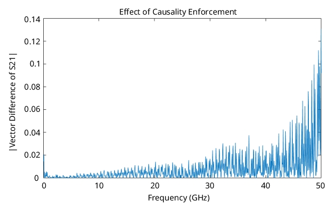
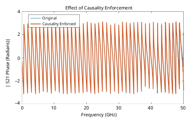
The corrections in this category also tend to be small and they are largest often at the higher frequencies. The plot in Figure: Vector Difference Caused by Causality Enforcement shows the vector difference of S21 between original and enforced data on a mismatched line of modest insertion loss (~8 dB at 50 GHz and 50 GHz of measurement bandwidth). The change is not visible on the magnitude of S21 in this example but the alteration can be seen in phase Figure: Actual S21 Phase Data With and Without Causality Enforcement as the distortions in phase have more of an effect on the temporal distribution of energy.

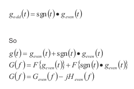
The enforcement process starts by coercing the imaginary part to have the desired relationship to the real part (there is some flexibility on what is a ‘fixed’ property that we will return to). To have zero energy before t=0, the time domain (impulse) function must have an odd part that will cancel the even part correctly:

Where Heven denotes the Hilbert transform has been applied (the Fourier transform of a time function with the sign function applied is a working definition).

Now, another conclusion of causality is that the negative frequency components of the response are the conjugates of the corresponding positive frequency components. This implies that the real part of the frequency response is exactly the even portion. Thus the enforced result is simply related to the Hilbert transform of the real part of the data.

From an energy conversation point-of-view, it may be preferable to keep the magnitude of the parameter fixed instead of the real part and this is presented as the default configuration. This fixing of the magnitude is easy to accomplish since we can simply scale the result above by a real function (normalizing magnitude).

As in passivity enforcement, the coercion process does change the data so if the changes are large, it is generally advised to look into possible measurement execution issues (use a VNA with wider bandwidth, calibration components or method choice, cable drift, connection repeatability, etc.) to see if the measurement could be improved instead.