This specialty sweep type is a hybrid of the power sweep and linear frequency sweep types discussed earlier. The application is used to evaluate compression points across multiple frequencies without having to setup power sweeps individually at each frequency. The nomenclature and the meaning of the displays require some interpretation different from other measurements, so some care is required.
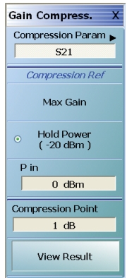
GAIN COMPRESSION Setup Menu for Power Sweep (Swept Frequency)
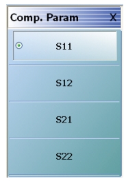
The compression parameter (Figure: COMP. PARAM (COMPRESSION PARAMETER) Menu), which must be a ratioed S-parameter, is the variable that is used to find the compression point (S21 is usually used for this role).
COMP. PARAM (COMPRESSION PARAMETER) Menu
Note that the compression will be based on an S-parameter and cannot be user-defined.
The compression parameter is a per-trace selection; that is, every displayed response parameter can be referenced to compression of a different S-parameter. Commonly S21 will be used for the compression parameter in all cases but the flexibility is available.
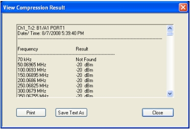
The desired plot variables, which are set up in the usual way with trace and response menus, are then evaluated at the power producing the indicated compression level in the compression parameter. The “view result” button will display (vs. frequency) the active trace parameter at which the desired compression occurred. This display will be in tabular form in a separate dialog (Figure: VIEW COMPRESSION RESULT Dialog Box).
VIEW COMPRESSION RESULT Dialog Box
The dialog shows the value of the active trace parameter at the desired compression point. If the active trace has a two graph display (e.g., log magnitude and phase), there will be a third column added.
Power-Sweep Swept Frequency Example
To help understand these concepts, consider an example. We have an amplifier connected in the usual forward direction (S21 > 0 dB) and we wish to know the output power and the output match when at the 1 dB gain compression point at a few frequencies. Assume that sufficient attenuation is employed to prevent VNA compression and that all needed calibrations have been performed.
• At 1 GHz:
• S21
• = 10 dB at –10 dBm input (low power) and
• = 9 dB at +1 dBm input
• B2/1 (output power)
• = 0 dBm for –10 dBm input and
• = 10 dBm at +1 dBm input
• S11
• = –15 dB at –10 dBm input and
• = –17 dB at +1 dBm input
• At 2 GHz:
• S21
• = 12 dB at –10 dBm input (low power) and
• = 11 dB at +3 dBm input
• B2/1 (output power)
• = 2 dBm for –10 dBm input and
• = 14 dBm at +3 dBm input
• S11
• = –17 dB at –10 dBm input and
• = –18 dB at +3 dBm input
• At 3 GHz:
• S21
• = 7 dB at –10 dBm input (low power) and
• = 6 dB at –1 dBm input
• B2/1 (output power)
• = –3 dBm for –10 dBm input and
• = 5 dBm at –1 dBm input
• S11
• = –10 dB at –10 dBm input and
• = –8 dB at –1 dBm input
The compression points based on the compression parameter of S21 (input power referred) are as follows:
• 1 GHz: +1 dBm
• 2 GHz: +3 dBm
• 3 GHz: –1 dBm
Since output power and output match at 1 dB compression are of interest, one would select b2/1 and S22 as the display parameters. In this sweep type, those parameters will be evaluated at the above power levels established by the compression measurement. A plot of |b2/1| would then show:
• 1 GHz: 10 dBm
• 2 GHz: 14 dBm
• 3 GHz: 5 dBm (assuming a power out graph type is being used and a receiver cal is in place)
A plot of |S11| would show:
• 1 GHz: –17 dB
• 2 GHz: –18 dB
• 3 GHz: –8 dB (assuming a log magnitude graph type)
Any of the normal S-parameters or user-defined parameters can be selected as the display variables (just as in any other sweep type). Those most commonly used are the S-parameters (to represent amplifier quasi-small-signal behavior at the point of compression), an un-ratioed parameter to represent output power at compression (often |b2/1|), and an un-ratioed parameter to represent input power at compression (often |a1/1|). Again, a receiver calibration is required for the representation of absolute power (input or output) and this is discussed in detail in another chapter of this measurement guide.
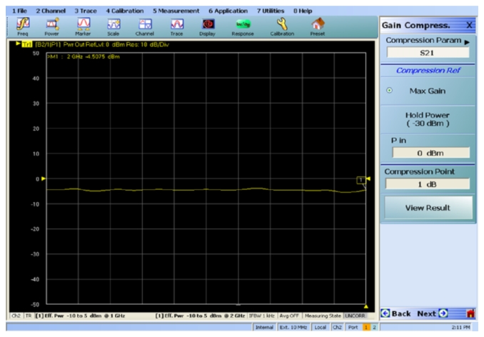
The plot resulting from an example measurement is shown in Figure: Example Plot from Power Sweep with Swept Frequency. Here the frequency sweep range was 1-2 GHz while the power sweep range (at each frequency point) was -10 to +5 dBm. The display parameter is output power (|b2/1|) while the compression parameter is S21.
Example Plot from Power Sweep with Swept Frequency
Some points of note:
• Frequency range is setup using the normal frequency menu. The only constraint is that a maximum of 401 frequency points can be used.
• The power sweep range is setup as with CW power sweep. The usual limits on power points apply.
• If one wants to look at the actual gain compression curve (|S21| vs. power for example), set up a 2nd channel, since power sweep (CW) and power sweep (swept) cannot be combined in the same channel.
• S-parameter calibrations are basically handled as in linear frequency sweep. If performed while in this sweep type, they will be conducted at the start power. The same error coefficients will be applied at all power levels. If the calibration was performed in linear frequency sweep, the point count will be coerced in this sweep type to get under the 401 point limit (interpolation will be used if it is active).
• Receiver calibrations are normally required for accurate plots of output power and can be performed in this sweep type or in other sweep types as long as the appropriate frequency range is covered.