In addition to the broadband measurements described in the previous section, the 3739x test set supports a number of different banded mmWave measurement setups that are described in this section.

The broadband selections allow operation from the low-frequency limit of the instrument (70 kHz or 10 MHz depending on Option 70 presence/absence) to the upper limit of the mmWave module.

For use of banded versions of the 3743x mmWave modules (described above and sold as the 3744x), the appropriate frequency band selection should be made from the NLTL MODULES BANDS menu. These modules allow operation in 145 banded GHz range or extended E (54-95 GHz) or extended W (65 GHz to 110 GHz) bands and are convenient for purely waveguide-based applications. The corresponding options on the VNA are 082 (without step attenuators) and 083 (with step attenuators). All of the 08x options are mutually exclusive.

External OML/VDI mmWave modules can also be selected for operation. Much like the 3738 test set-based systems, OEM mmWave modules are used, except the internal VNA sources are used to drive the modules and additional leveling capabilities are enabled. The mmWave module selection is done from the mmWAVE WG BANDS menu.

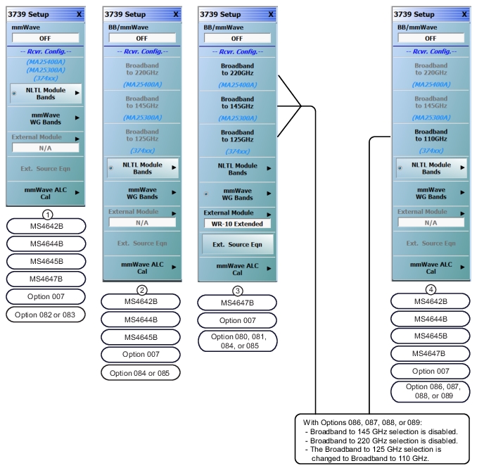
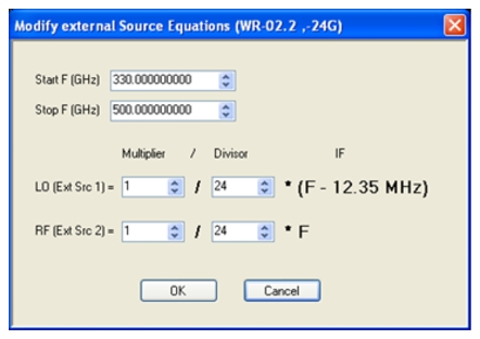
The 3739-based setup is enabled from the RCVR CONFIG menu and has additions (see Figure: 3739-based SETUP Menu) relative to the 3738 setup for the E-and W-banded solutions, as well as for a leveling calibration that will be discussed shortly. The EXTERNAL EQUATION dialog has the same structure as for the 3738 setup, and an example for a WR-2.2 (24 GHz) module is shown in Figure: Example EXTERNAL SOURCE EQUATION Dialog Box for a WR-2.2 Setup.

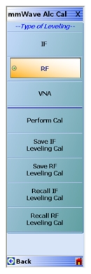
The 3739-based mmWave systems have some power control options available that are not present on the 3738-based systems and they are illustrated by the mmWAVE ALC Cal menu shown in Figure: mmWAVE ALC CAL Menu.

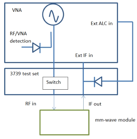
To understand the leveling/power control options, consider the very simplified block diagram in Figure: Simplified Block Diagram of a 3739-based mmWave Setup. The key point is that there are multiple locations to sample the power, but because of the very high frequencies involved, there is potentially no one ideal location.

In the ‘VNA’ mode, the standard VNA ALC calibrations are used with the existing detection system in the VNA so that the power menu settings correspond roughly to the actual RF levels being delivered to the 3739x test set. One can then have a general idea of the levels driving the module, and may know the corresponding mmWave output power levels based on data from the manufacturer. The leveling loop is closed, but in this mode the instrument has no knowledge of the relationship between mmWave power levels and the instrument settings.

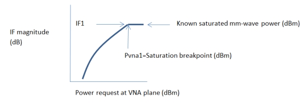
In the RF leveling mode, the same detection circuitry is used as in the VNA mode, but now a means of relating the actual mmWave power levels is available. Because of the paucity of readily-available power measurement methods in these higher frequency ranges, the method used is somewhat indirect, but relies on the established linearity of the measurement system. The concept is illustrated in Figure: RF mmWave Leveling Concept. From the manufacturers’ measurements (often based on quasi-optical or other techniques), a value is generally known for the saturated mmWave power. The saturation breakpoint can be found by locally sweeping the VNA RF power until the measured IF power leaves saturation (Pvna1). The IF reading can be noted at this point (IF1) and it can be linked to the known mmWave saturated power. Now the VNA plane power can be dropped and the IF magnitude recorded as a function of this setting. Based on the known receiver linearity, we can now link the IF changes to the mmWave power level (note this is only done during the calibration step. The leveling is based on finding the needed VNA setting to get the requested mmWave power level, and then relying on the VNA leveling loop). So if the IF level has decreased to IF1-10 dB at some input level Pvna2, then we can state the mmWave power is Psat-10 dB with some reasonable level of uncertainty. The concept is to level on the VNA power plane while establishing a link to the mmWave power so that user entries can be in the latter form.

Since this leveling method only relies on the detection system at the VNA plane, it is useful for all measurement classes including converter and IMD measurements. Because it is leveling prior to the multipliers, it is less stable than the IF leveling to be discussed next and will provide a lower level of long term accuracy.

The calibration is accomplished using the dialog shown in Figure: mmWAVE ALC CALIBRATION Dialog for a Single Frequency Point of RF Calibration on Port 1. The concept is that the saturated power is known at some frequencies in the band and the user is allowed to enter those values discretely. When the calibration is executed, the above power sweep and iteration scheme is executed individually at each of the frequencies requested. Note that Port 1 and Port 2 calibrations are separate since modules are rarely identical. 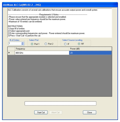When the calibration is completed, the calibration may be saved and recalled later using the buttons shown in Figure: mmWAVE ALC CALIBRATION Dialog for a Single Frequency Point of RF Calibration on Port 1.

The IF leveling scheme relies on sensing the IF amplitude coming out of the module directly and using that IF signal as the leveling signal. This requires that an IF be present on the reference channels so it is not appropriate for mixer or IMD measurements. Since the IF is derived post-multiplication, however, it is much more stable over time and temperature than is the RF leveling scheme discussed before. The block diagram of Figure: Simplified Block Diagram of a 3739-based mmWave Setup still applies except now the Ext ALC path shown is used for leveling.

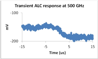
The calibration proceeds in the same way as discussed for the RF leveling scheme and the same dialog is used (with different button selections). In both cases, since the leveling is analog, it is very fast so that the DUT rarely sees transient power spikes that can occur under purely software leveling schemes. The detected transient response time for one measurement is shown in Figure: Example Transient Response of the mmWave ALC System and illustrates that a ~5 dB power request step is resolved in a few microseconds in an overdamped manner.

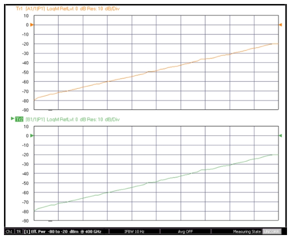
Both leveling schemes enable power sweeps as well as finer power control when sweeping frequency. Both modes of control can be useful for active device measurement or for other RF-sensitive or potentially non-linear situations. An example of a power sweep at 400 GHz is shown in Figure: Example Power Sweep Measurement to illustrate the range that may be possible.