The noise figure measurement process consists of a few relatively straightforward steps:
1. Measurement of DUT gain or S-parameters (over an appropriate frequency range and at an appropriate power level as discussed before)
2. Perform an optional user power calibration over the frequencies of interest to optimize receiver calibration accuracy
3. Physical configuration for the noise measurement (discussed in the previous section)
4. Basic setup (frequency range, number of points, type of device)
5. Receiver calibration (transferring the traceable power accuracy to the receiver)
6. Noise calibration (measurement of the receiver noise power so it can be removed from the calculations)
7. DUT measurement
The first three items have already been discussed. A few more details are in order on the gain/S-parameter measurement comment.
Gain/S-Parameter Data
The gain/S-parameter data should be acquired on a frequency range containing the desired noise figure frequency range. The same frequency points need not be used (although that may be desired if the gain changes rapidly with frequency) as interpolation will be invoked. Extrapolation will also be used if needed, but this is not advised for accuracy reasons.
S-parameters should be saved in the S2P file format and they will be loaded in the noise figure application. A full 12-Term calibration is advised for optimal accuracy and to enable the use of the more correct available gain terms, but data from normalization-only calibrations will also be accepted.
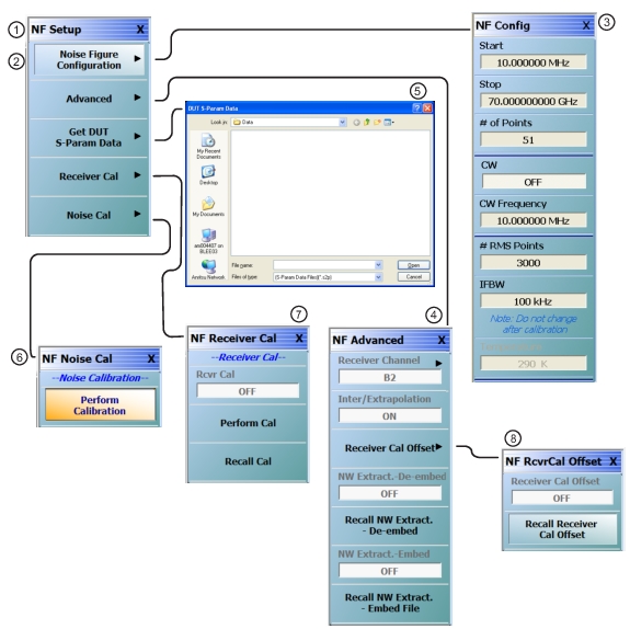
11. PERFORM RECEIVER CAL dialog box. Provides access to previously saved receiver calibration RCVR files.
Note
When the instrument changes the VNA application mode from Transmission/Reflection to Noise Figure, the instrument resets to the default settings for that mode.
The default Noise Figure trace condition is a single trace and Noise Figure (LogMag) response.
The default Transmission/Reflection condition is four traces, S11 (Smith Chart), S12 (LogMag + Phase), S21 (LogMag + Phase), and S22 (Smith Chart) responses.
Most of the setup parameters are self-explanatory. Some of the more noise-specific items
• Number of RMS Points
The number of measurements used in the noise power computation.
• Temperature
This is nominally the temperature of the cold termination used during the measurements and defaults to 290 K. The IEEE definition specifies this temperature, which may be different from the physical termination temperature. For reference:
• 290 K = 17 ºC (62.6 ºF)
• 0 K = −273.15 °C (−459.67 °F)
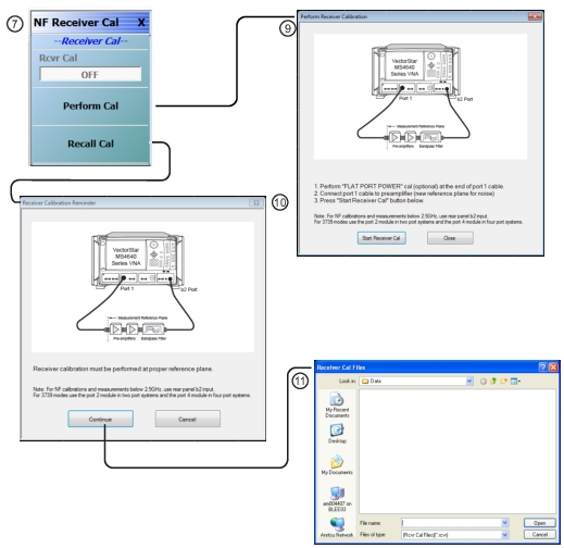
The receiver calibration in Step 5 is performed by simply connecting a cable from the source (usually Port 1) to the receiver input plane as suggested in Figure: Noise Calibration Step 5. The power calibration discussed earlier and in Step 2 should ideally be performed at the end of this cable. The receiver calibration, as discussed elsewhere in this document, measures the receiver parameter and forces it to match the calibrated power level. Uncertainty addition may come at this point due to mismatch between the source and receiver and due to any residual nonlinearity in the receiver. These points will be discussed in more detail in the uncertainties section.
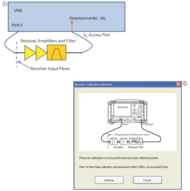
Noise Calibration Step 5
1. The receiver calibration (Step 5) is illustrated here as a schematic view. Note the VNA connections at Port 1 and the b2 Access Port and also the Receiver Input Plane.
2. The equivalent pictorial view is shows in the RECEIVER CALIBRATION REMINDER dialog box.
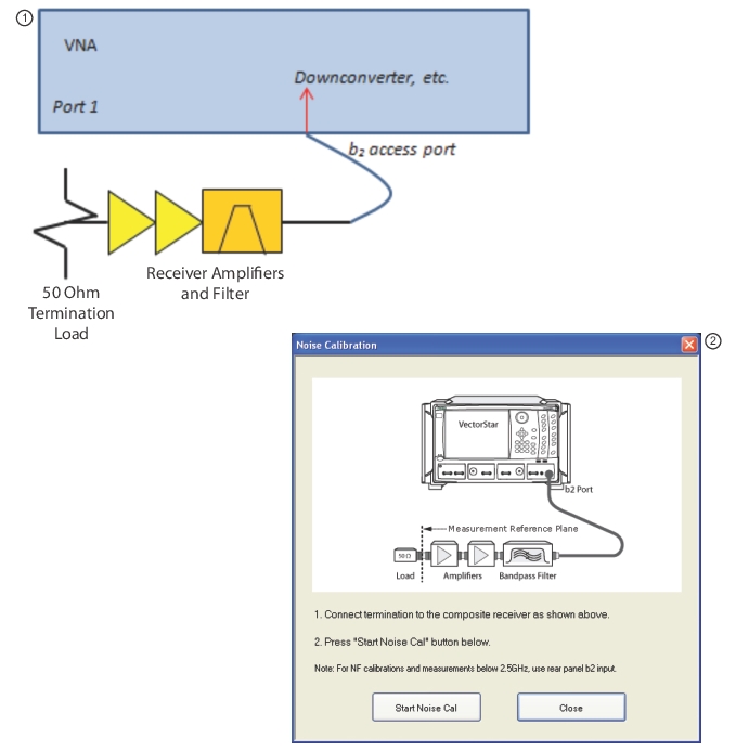
The noise calibration in Step 6 is even simpler. Here one simply places the 50 ohm cold termination on the input to the receiver plane and allows the system to measure noise power. This is illustrated in Figure: Noise Calibration Step 6. Depending on how many frequency points are used, this may be the most time-consuming of the setup/calibration steps (allow on the order of 0.2 seconds to 2 seconds per frequency point depending on IFBW, averaging, and number of RMS points). If the frequency range is changed after calibration, interpolation and extrapolation of both the noise calibration data and DUT S-parameter data will be employed. Uncertainties may degrade, particularly if extrapolation is invoked by going outside the original frequency range of either step.
Noise Calibration Step 6
1. The noise calibration (Step 6) is shown here as a schematic view.
2. The equivalent pictorial view is shows in the NOISE CALIBRATION dialog box.
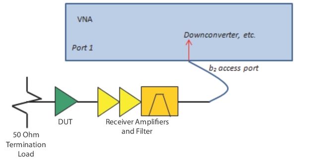
Step 7, the final step, is the measurement of the DUT itself and this is equally simple. The output of the DUT is connected to the receiver input plane and the cold noise source with a typical termination load of 50 Ohms is connected to the DUT input. This step is shown in Figure: Amplifier DUT Final Measurement Step.
Amplifier DUT Final Measurement Step
The final step, that of measuring the DUT (here illustrated as an amplifier), is shown here. Note the 50 Ohm Termination Load attached to the DUT.
Measurement Example
To integrate all of these concepts, let us consider an example measurement.
• DUT 1.7 to 2.4 GHz
• With an average gain of 12 dB
• A nominal noise figure of 0.8 dB.
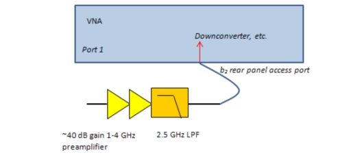
This is a challenging measurement in some sense in that the noise figure is relatively low and the gain is not very high. We will proceed with an IF Bandwidth of 1 kHz and 3000 RMS points and no averaging. The receiver structure is annotated in Figure: Example of Measurement Receiver Structure. The compression point of this structure is about –10 dBm which should easily avoid linearity issues. The power calibration and receiver calibration will be performed at –60 dBm. The input match of the preamplifier structure was better than –20 dB and the noise parameter Rn was small enough that a 0 dB source match only results in a 0.1 dB receiver noise figure deflection. Since all frequencies are below 2.5 GHz, the rear panel b2 access port is used.
Example of Measurement Receiver Structure
The example measurement receiver structure is shown here.
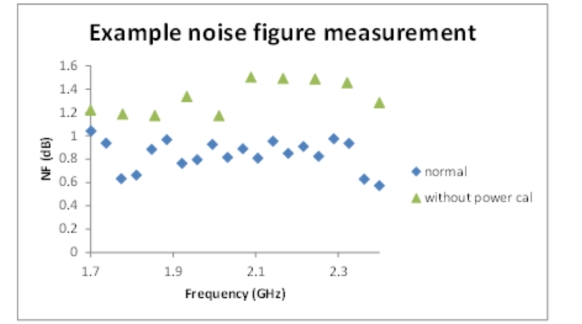
Because the noise figure is low, accuracy throughout the receiver calibration step is important since those errors will propagate roughly on a dB-for-dB basis. Since the basic ALC factory calibration has a nominal uncertainty of 0.5 dB to 1 dB, using this in lieu of a user power calibration could have a significant impact on this measurement. The difference in results is shown in Figure: Receiver Calibration Example with and without a Power Calibration.
Receiver Calibration Example with and without a Power Calibration
The example measurement is shown here with and without a power calibration preceding the receiver calibration.
For another example, a mixer will be considered. In this case, the DUT has a fixed IF of 70 MHz and an RF range of 2 GHz to 2.5 GHz (and the LO is below the RF). The mixer setup dialogs discussed earlier make this setup straightforward. The conversion gain of the DUT is approximately 10 dB. The basic measurement parameters are the same as in the previous example. A different low pass filter is used to avoid LO leakage corrupting the receiver response (the DUT in this case is already well-filtered but it is reasonable practice). A preamplifier with a 10 MHz low end was used for this setup.