As was suggested in the previous section, there are many different ways of making mixer measurements and many different calibration approaches. The purpose of this section is to explore some of the options and how they might perform under various circumstances.
Some of the mixer measurements described in the previous section (match and isolation) are essentially simple S-parameter measurements that have been discussed previously in this guide. The match measurements are generally 1-port in the case of mixers (from a correction point of view) since the other ports of the mixer are operating at different frequencies. Depending on the isolation of the mixer, there can lead be some load match dependencies and some confusion in the meaning of the practical match of the mixer (see Figure: Actual Match Dynamics).
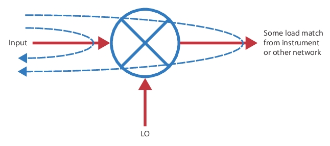
Actual Match Dynamics
An illustration of the dynamics of the actual match of a mixer is shown here. If the isolation of the mixer is poor and the load match at the input frequencies is poor, multiple reflections can make the actual match of the mixer (in system) worse than one might expect. This can also have implication in conversion loss measurements as will be discussed.
The newer measurement is really that of conversion gain/loss although it has been touched on in the Multiple Source Control chapter. The concept as discussed above is power transfer from input to output but since the frequencies are different, a classical ratioed S-parameter is not possible (a1 is at the input frequency and b2 is at the output frequency). There are several ways to handle this.
Normalization
This is a scalaresque approach where the receiver is calibrated for absolute power and the input power is calibrated absolutely. This allows one to measure the power received at the output and calculate conversion loss/gain based on knowledge of the input power. This is using the VNAs narrowband receiver so one is not also measuring spurs and leakage that one may be doing with power meter techniques and is hence more accurate than those approaches. Match is, however, neglected and can reduce accuracy. The ports can be heavily padded to reduce any match-related error. Also, group delay of the DUT is unavailable with this method but it is the simplest approach and may be most practical in millimeter wave frequencies or in complex media. The measurement is illustrated in Figure: Normalization Method of Conversion Loss/Gain.
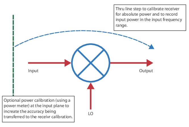
Normalization Method of Conversion Loss/Gain
The normalization method of conversion loss/gain measurements is shown here. A thru line is used to establish the input power to the DUT (at the input frequencies) and to calibrate the receiver for absolute power (at the output frequencies). Match is neglected and padding of the ports (prior to calibration) is sometimes done to reduce mismatch effects of a poorly matched DUT.
Enhanced Match
This calibration approach combines power normalization with vector match correction to make a vector method that is still relatively simple to execute and provides better accuracy. The concept is illustrated in Figure: Enhanced Match Calibration and relies on multiple one port calibrations in multiple frequency ranges per port (input and output ranges) to correct for DUT match interaction with the ports and for port match interaction during calibration steps. The accuracy is better than that of straight normalization at the expense of some additional calibration steps. Group delay information is also not available with this method.
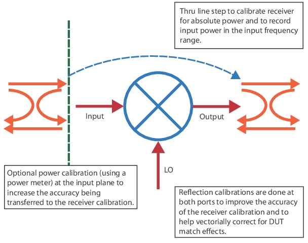
Enhanced Match Calibration
The enhanced match calibration is shown here. The ports are corrected for mismatch at both input and output frequencies so that match effects during both the DUT measurement and during the calibration steps can be corrected vectorially.
The principles of the enhanced match calibration are essentially the same as for the regular S-parameter calibrations covered earlier in this document. There are the obvious disparate frequency ranges involved and some assumptions are implicit that are worth discussing. The error boxes for the present problem are illustrated in Figure: Error Boxes for Enhanced Match Correction. The reflectometer terms have the frequency range explicit in their names. The transmission terms have the frequency conversion implicit in their definition (with a ~ to denote a variance from the usual S-parameter meaning in that now it applies to unratioed conversion).
The receiver calibration is corrected for the interaction of the input port source match and the receiving port load match (ports 1 and 2 in this description although that is not a requirement). This reflection term is of the form (1-ep1S*ep2L) and is done for both input and output frequencies. For the DUT correction, similar terms apply for the interaction of DUT S22 and ep2L_out and the interaction of DUT S11 and ep1S_in. As the isolation terms are included, this correction gets more complex but the form of the terms is similar.
Since only fundamental mixing terms are included, this correction can never be complete so the accuracy will be best when the device is operating more linearly (obvious on many levels), when isolation is high, and when the DUT is more unilateral (i.e., does not convert in both directions well).
A variant on this correction, termed “True Source Match,” uses a modified term (instead of ep1S_in) to help describe the input match interaction. This is helpful, particularly in mmWave mixer measurements, where the actual source match starts to diverge more from the ep1S term due to coupler placement. When this mode is enabled, an additional backward-looking measurement is performed during calibration to better characterize the source match that the DUT actually sees.
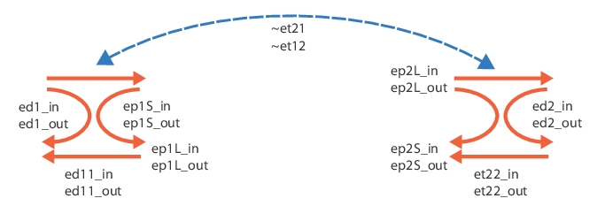
Error Boxes for Enhanced Match Correction
The error boxes for the enhanced match correction are shown here. Port 1 is used as the input and Port 2 as the output in this figure but that is not a requirement.
Broadband Enhanced Match Cal
Commonly SOLT, SSLT or SSST calibration cores are used for enhanced match calibrations (or variants using the hybrid calibration processes) but, if 1 mm or 0.8 mm coaxial components are employed, it may be desirable to combine SOLT and SSST calibrations as is done in conventional, broadband S-parameter measurements. In these ‘merged’ calibrations, the open-short-load or triple-offset-short algorithm is employed depending on if the current frequency is above or below a breakpoint frequency (default is 67 GHz for 1 mm and 80 GHz for 0.8 mm calibration kits). This same merged approach can be used with enhanced match calibrations and the frequency sorting will be performed on both input and output ports.
Reference Mixer
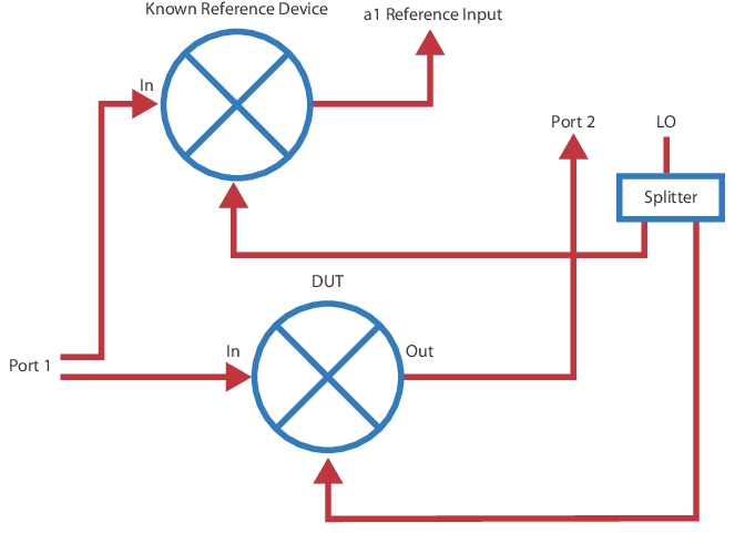
One way to get back to a ratioed measurement is to also place a converter in the reference channel (a1 often). This requires one of the loop options (051/061/062) but allows for a S21 (or similar) measurement to be made on a mixer and hence allow group delay extraction. The simplest approach is to use a very broadband (relative to the DUT) mixer that is well-padded to act as the reference mixer so the correction for its effects is a simple normalization. The concept is shown in Figure: Reference Mixer Approach.
The reference mixer sequence is not explicitly supported in the wizard setup systems but is compatible with it. The reference mixer must obviously support at least the frequency plan of the DUT but ideally is very broadband. The LO is shown as split in Figure: Reference Mixer Approach but another synthesizer (as long as it is locked to the same time base as the instrument) can also be used. Indeed, a harmonic mixer with a different multiplier can be used as the reference but multiple source control will generally be needed for this effort (see Multiple Source Control (Option 7)).
Reference Mixer Approach
The reference mixer approach is shown here. The port definitions can be changed as before.
Embedding/De-embedding
A more complex approach is to characterize the reference mixer and then to de-embed its effects using the embedding/de-embedding engine discussed in a previous chapter. The parameters of this mixer can be found using the NxN method (see the next chapter) or using network extraction (Type B discussed elsewhere in this guide).
NxN
A fourth method, also recreating a ratioed measurement, is termed NxN and is discussed in more detail in the next chapter. The idea here is to use a characterized mixer to reconvert the DUT output frequency back to the input. This does not require a loop option but does require some care in handling the image and match at the interface between the DUT and the characterized mixer (usually with a simple filter and pads). Accuracy is approximately the same as with the previous two methods.