Option 31 introduces a second source into the MS464xB structure which has applications for mixer measurements, true mode stimulus measurements for differential/common-mode circuits, IMD and other two-tone measurements, and faster multiport measurements, etc. This particular option only introduces the second source which drives port 2 of a 2-port instrument. This section explores the basic structural and performance changes of the instrument, how common measurements might be configured, and the implications of more complex setups.

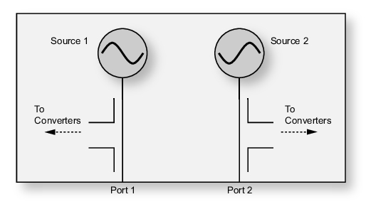
The block diagram illustrated in Figure: Dual Source Option 31 Block Diagram (simplified) shows what one would expect: parallel signal generation structures feeding two independent ports. Like the rest of the MS4640 family, there are separate paths for above and below 2.5 GHz. Relative to the non-Option 31 system, a transfer switch has been removed so that the two sources independently drive their ports. Everything in the source chain (including high band/low band components and multipliers) is replicated.

 

Option 31 removes the transfer switch, which enables higher port powers and more drive flexibility for applications such as mixer and multi-tone measurements. From a standard S-parameter measurement point-of-view, we must introduce the concept of an ‘inactive’ source. When, for example, Port 1 is driving in an S11 measurement, we do not want Port 2 driving to retain the definition of the S-parameter. As there is no longer a switch in position to block that source, it must be powered down as much as is practical and tuned to an innocuous place. The ‘safe’ place is possible since cross-aligned filters can be used to minimize any signal leakage. Fully powering down the source would not be advisable for reasons of measurement stability and speed. In normal S-parameter modes, this configuration is handled automatically for the user so nothing separately must be done; the S-parameter measurement acts as if the option was not present. When in multiple source mode, however, it may be desirable to take manual control of the process. The use of multiple source control (Multiple Source Control (Option 7) of this measurement guide) also requires the concept of ‘active’ and ‘inactive’ sources.

When in standard S-parameter mode and Port 1 is driving, then the state is {source 1 active, source 2 inactive}; when Port 2 is driving, the state is {source 1 inactive, source 2 active}.

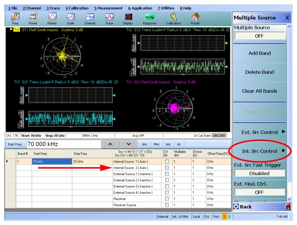
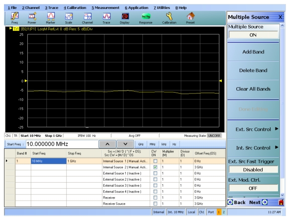
The multiple source setup screens change somewhat since the second source is completely independent. The new setup screen is shown in Figure: Multiple Source Setup Screen (instrument with Option 31). The internal second source entries function exactly as those for the first internal source as discussed in the multiple source Multiple Source Control (Option 7) of this guide. The new function is that of internal source control (see submenu in Figure: Internal Source Control Menu) which is a parallel of the external source control submenu that exists without Option 31.

The second internal source equation is an obvious and necessary addition. The Int. Src. Control button is added for this option and leads to the menu of Figure: Internal Source Control Menu.

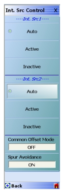
The internal source control submenu is shown here that allows one to independently activate or deactivate the two internal sources.

The ‘Auto’ state is how the sources behave in Standard receiver mode: the source is on-frequency and driving at requested power if that port needs to be driving for the given measurement. If, for example, all traces and applied calibrations are based on Port 1 driving, then Source 2 will always be inactive. If the user calibrations or the trace selections cover both ports driving, then sequentially the system will be in the following two states:

The double ‘Active’ state is useful for mixer and IMD measurements that will be discussed, while the double ‘Inactive’ state is useful when only external synthesizers are being used for a measurement. All selections are independent for the two sources so there are nine allowed permutations.

The nine possible internal source state configurations within multiple source control (with Option 31) are shown in Table: Internal Source State Configurations.

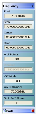
Additionally, when both sources are available and at the same frequency, relative phase control between them makes sense and a phase entry field applies on the Frequency menu as shown in Figure: Frequency Menu. This control is only available if both sources are active and at the same frequency. A factory calibration of phase applies in this case and is referenced to the test ports. When one needs the phase control at a more remote reference plane, it is important that equal length (in the electrical sense) paths be used on the two ports.

While phase control could be offered if both sources are active but the frequencies are not the same, the interpretation of the data becomes much more difficult as does a calibration, so phase control is not offered in this case. This is a precursor to the true mode stimulus functionality of Option 043 that is discussed in a later section. The phase control allows the direct measurement of phase-sensitive DUTs such as IQ modulators, certain power amplifiers, and other balanced active structures.

In Figure: Frequency Menu, the phase control entry field is shown for use in the cases when both sources are driving. The title of the entry box will show ‘Inactive’ if both sources are not turned on and at the same frequency.

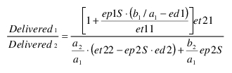
The factory phase calibration is an important concept, particularly with regard to its reference plane placement—at the test ports. If equal length cables are used (to within needed tolerance), then reasonably phase-accurate stimulus can be applied to sensitive DUTs and for cases such as IQ modulators. To measure the phase relationship, very linear and sensitive receivers are already available within the instrument, but we must remove the effects of path and match asymmetry in order for the phase calibration to be precise. Fortunately, this concept is already implicit in the user RF calibrations performed for ordinary measurements in the VNA (the directivity, tracking, and match error coefficients contain just the information needed). If both ports are terminated, then the actual delivered signal ratio (between the two ports) can be quickly calculated from the following (where the error terms were described in Calibration and Measurement Overview of this guide):

This equation then forms the basis of a factory calibration algorithm to get the desired delivered phase difference between the ports. With terminations connected, the indicated a1, a2, b1, and b2 parameters are measured and Equation 26‑1.   is used to calculate what the delivered phase to the reference plane actually was. The phase registers can then be adjusted to provide the correct phase at each frequency. This set of phase register settings forms the calibration.

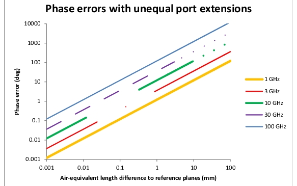
Variations of this equation are used for different port pair combinations. An obvious question is what level of length matching is required for a given phase error and a given frequency. This relationship is shown in Figure: Phase Error for Different Line Length Differences in terms of air-equivalent line length difference. For other media, multiply the physical length difference by the square root of the effective permittivity (for media such as coax cables, microstrip or coplanar waveguide in fixtures, etc.). For rectangular waveguide, the air-equivalent difference can be computed using the propagation constant [1]. As would be expected, the required care in length matching is a direct function of the frequency ranges involved for a given tolerable phase error.

On the subject of the factory phase calibration and its accuracy, two additional toggle buttons from Figure: Internal Source Control Menu require discussion. The factory phase calibration is performed over a certain frequency list and interpolation is used to get to the frequencies in use as discussed. The operating mode of the hardware during calibration and measurement will have some bearing on the accuracy of that interpolation, since the interpolation process requires some knowledge of how the sub-synthesizers in the system are programmed regarding their phase transitions and other properties. Two aspects of the factory phase calibration are ‘Common Offset Mode=On’ (which describes how some of the internal synthesizers are referenced) and ‘Spur Avoidance=Off’ (which means little effort is put forth in realigning internal synthesizers to avoid interaction spurs with the DUT.

Spur avoidance is normally turned off in multiple source mode since many of the spurs generated by a DUT, such as a mixer or multiplier (which are the typical multiple source mode DUTs), overwhelm the internal synthesizers and cannot be corrected. By maintaining these settings (Common Offset Mode=On and Spur Avoidance=Off), the best possible interpolation success of the factory calibration is ensured. There may still be small errors in places due to synthesizer frequency hops. If the other modes are needed (such as Spur Avoidance=On for a near-noise-floor measurement with a non-spur producing DUT or Common Offset Mode=Off for a frequency converting DUT), then interpolation will still be attempted, but it may be less successful near some source transitions (such as the particularly dense < 5 GHz system frequency). A key aspect of Common offset mode is that it can only be used when the base source frequencies and LO frequency are within ~320 MHz of each other when referenced to the 10 to 20 GHz frequency range (~160 MHz in the 5 to 10 GHz range, ~80 MHz below 5 GHz, ~640 MHz in the 20 to 40 GHz range, and so on).

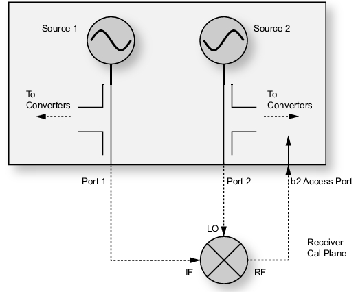
To illustrate basic Option 31 control via multiple source mode, consider an upconverter measurement where internal Source 1 will be used as the IF stimulus (ranging from 0.01 GHz to 1 GHz) and internal Source 2 will be used as the LO (fixed at 3 GHz). The RF output of the DUT will be fed directly to a b2 loop input. In this case, the RF will be ranging over 3.01 to 4 GHz. The setup is shown in Figure: Mixer Measurement Setup Example and the multiple source screen is shown in Figure: Multiple Source Screen for the Example Mixer Measurement. Both sources are put in the Active state since we want them both to always be driving (with careful selection of the response parameters, one of the sources could have been left in the Auto state). A receiver calibration (Receiver Calibrations of this measurement guide has more information) was used for calibration and the conversion loss of the passive upconverter is also shown in Figure: Multiple Source Screen for the Example Mixer Measurement. More details on mixer measurement calibration approaches are discussed in Mixer Setup and Measurement of this measurement guide. For the desired drive levels, the port powers were uncoupled so that Source 2 could be set at the required +7 dBm for this measurement and Source 1 could be set to the desired 0 dBm.

 

Additional points to consider when using Option 31:

The broadband and millimeter wave options (Broadband/mmWave Measurements (Option 7, Option 8x) of this measurement guide) continue to be available with the dual source modes and most of the operational aspects will be available. In 2-port systems based on the 3739x test set, however, simultaneous source drive in the millimeter wave bands is not possible because of how the RF is routed. In 4-port systems based on this test set, however, simultaneous (both sources Active) drive is allowed. The relevant options for configuring for use with the 3739x test set are Option 084 (when the base VNA does not have loops) or Option 085 (when it does have loops). A second RF tap is provided with Option 084/085 (relative to Option 080/081 for MS4647B, and relative to Option 82/83 for MS4642B, MS4644B, and MS4645B); and this is used for dual drive in the 4-port cases. When used in a 2-port configuration, assembly is done as it is for a non-Option 31 VNA with the RF1 spigot connected to the 3739x test set. When used with a 4-port system, RF1 on the VNA is connected to the controlled test set and RF2 is connected to the controlling test set. LO, IF, and Control connections are unchanged.

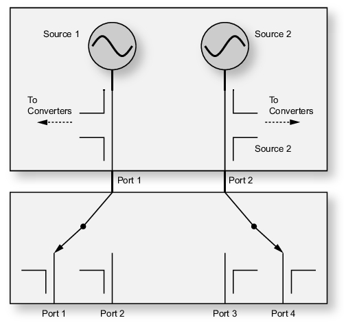
When connected to the 4-port test set (MN469xx), dual source drive is also possible. If sources are in the Auto state, the 4-port measurements will proceed as they do in single source instruments. If both sources are Active, then two of the four ports will be driving. Because of the partial switching fabric, not all permutations of driving ports are possible (1-3, 1-4, 2-3, and 2-4 are possible; 1-2 and 3-4 are not). This concept is illustrated in Figure: One Dual Drive Configuration when Using the 4-port Test Set.

 

The port power controls are unchanged when adding Option 31. Without Option 31, two calibrations were stored, one for each port, since the RF paths were different. With Option 31, two calibrations are again used but now they pertain to entirely different source paths. The power settings are coupled by default (i.e., power levels change together), but this can be turned off. User power calibrations (discussed in Receiver Calibrations of this guide) also apply to the two source paths independently.