DifferentialView™ is True Mode Stimulus (TMS) and requires the Option 31 dual source architecture. As has been discussed in the literature (e.g., [2]-[3]), there are certain measurements of certain differential devices where it is critical that the device be driven with true differential and/or common-mode signals. That is, the superposition method discussed in Multiport Measurements is not adequate. There is a nonlinear phenomenon that can occur when the early stages of the DUT are compressing in an unbalanced fashion. If the DUT is not compressing or if the apparent front-end compression occurs in a balance fashion, then true mode stimulus and single-ended stimulus produce the same results [2]. The purpose of this option and this section is to cover the other case.
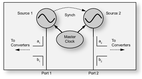
Option 43, working with the dual sources of Option 31, provides a phase-calibrated stimulus for this situation. The option integrates drive changes with the user RF calibrations to ensure an accurate phase relationship is delivered to the DUT. The main change relative to the usual configuration of Option 31 is that the dual sources are phase synchronized and the phase registers programmed according to a calibration process. This concept is illustrated in Figure: Phase Control and Synchronization Concept of Option 43. Hardware clocking and synchronization ensure repeatable phase programming and measurements on the measurement channels will enable real-time correction of the phase angles as needed.
Phase Control and Synchronization Concept of Option 43
The factory phase calibration discussed in the Option 031 section may be adequate for some applications. In the class of unbalanced front-end compression relevant for this section, more is needed. Since the reflections of the DUT may be very unbalanced (particularly when it is experiencing unbalanced compression), the net phase relationship delivered to the DUT may be different from the incident phase relationship. Such a delivered phase discrepancy can significantly change the response of the device if it is sufficiently nonlinear [2]. A solution to this is to adjust the incident phase relationship so that the delivered phase relationship is at the desired value based on the S-parameters of the DUT. This is the core of Option 43 along with phase sweep features.
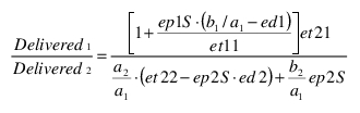
A natural approach is to build this into the user RF calibration routines since the S-parameters and needed error coefficients are already available. This is something of an extension of the factory calibration discussed earlier except now the reflections are arbitrary. The phase relationship would be set up based on the factory calibration to get the incident arrangement correct, and then the delivered relationship can be computed from the below (where a1, a2, b1, and b2 are measured when the DUT is driven with the desired common-mode or differential signal).
Equation 26‑2.
The phase and amplitude drives are then adjusted as necessary to get the correct delivered signal relationship. Obvious variations of Equation 26‑2. are used for different port pairs in a 4-port system.
The application of the calibration then proceeds normally. The differential and common-mode measurements are made (subject to any user requested phase and amplitude offsets), the single-ended parameters calculated from those measurements, and the calibration error coefficients applied. All calibration algorithms are supported. It is important to note that the calibration is done in a single-ended sense (since the error terms are the same) so the same calibration is used for both single-ended and TMS measurements. If one is in TMS mode when a calibration is started, the system will automatically switch to single-ended mode for the calibration and then revert to TMS at the conclusion of the calibration. This duality of the calibration, applying to both single-ended and TMS modes, makes it very convenient to switch between them. Note that interpolation is very problematic for TMS due to the phase correction requiring very good error coefficients, so interpolation is not allowed when in TMS mode.
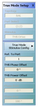
The main menu of the true mode stimulus application for a 2-port system is shown in Figure: Two Port True Mode Setup Menu. The main purpose of the menu is to give, at a glance, some of the most important TMS parameters (such a port configuration) and allow offset changes to be entered. The port reference is to help establish the sign convention. The phase and power offsets are applied to both the common-mode and the differential mode states when in TMS drive. When in single-ended but double-active drive (discussed earlier), they both apply to the static state at every frequency. If the phase sweep was active (available for CW only), the start and stop limits would be enterable here.
Two Port True Mode Setup Menu
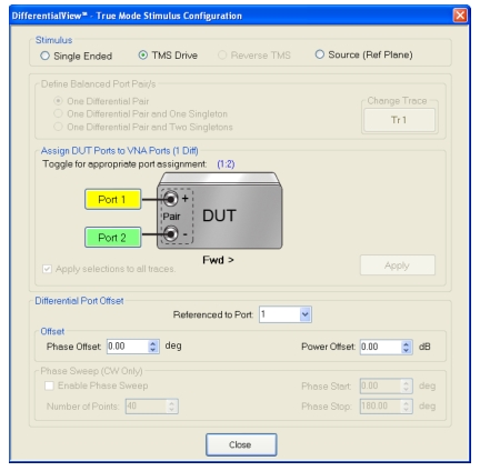
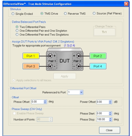
The configuration panel for True Mode in the 2-port case is shown in Figure: TMS Configuration Dialog (2-port case). The Single Ended state is the default and is exactly the standard VNA mode discussed before where multiple source controls can override. The Source (Ref Plane) selection turns on both sources (same frequency) and allows one to perform measurements without the phase correcting link to the user RF calibration (to be discussed), thus saving sweep time. The existing factory phase calibration is used and the phase and power offsets can be used for adjustment or manual correction. The phase sweep is available when in CW and can be useful for identifying null points and to balance the state of a variety of devices, and can be very useful as a troubleshooting tool (hence why the reduced sweep time in Source (Ref Plane) mode is helpful).
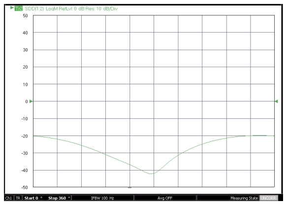
As an example of this, consider the measurement of the differential return loss of a balun-based device input stage; it may be interesting to see how centered the return loss null is relative to 180 degrees and how abrupt the change is with phase deviations from that value. Such a measurement result is shown in Figure: Example Phase Sweep Measurement. A full port RF calibration is generally required.
There is not much to the port assignment in the 2-port case except for providing the sign reference. The assignment can be changed by clicking on the port buttons.
TMS Configuration Dialog (2-port case)
Note
A full 2-port calibration must be applied for TMS drive and Source modes.
Example Phase Sweep Measurement
An example phase sweep measurement is shown here of the differential return loss (SDD) of a balun-based front-end. The match null in this case is roughly centered at 180 degrees as would be expected and the response is relatively broad.
In terms of measurements, single-ended responses can be plotted since they are the base result of the calibration process, but it is more common in TMS mode to use the mixed mode parameters SCC, SDD, SCD, and SDC for the 2-port case (see Multiport Measurements). As discussed in the pre-amble to this section, the single ended and TMS versions of these parameters will be the same for linear devices and some nonlinearly operating ones.
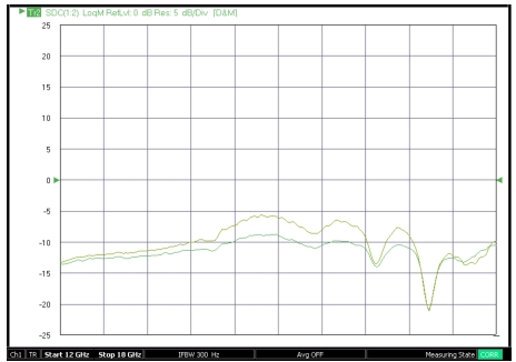
Measurement of Differential Input Match and Mode-converting Match
A measurement of differential input match (|SDD| at left) and mode-converting match (|SDC| at right) of a transimpedance amplifier is shown here in both single-ended and TMS modes. There is no appreciable difference in this case.
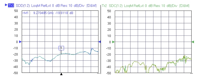
But another device shows a substantial difference with the two drive modes, partially because of a radically different common-mode behavior. In this case, the difference particularly shows up in reflected mode conversion and is displayed in Figure: Measurement of Mode Converting Reflection of a more Unbalanced Nonlinear Device. The absolute mode conversion is much higher than when a similar device is in a linear state and single-ended drive overstates the value by several dB.
Measurement of Mode Converting Reflection of a more Unbalanced Nonlinear Device
The measurement of mode converting reflection of a more unbalanced nonlinear device is shown here with single-ended data in the lighter, upper trace and TMS data in the darker, lower trace.
As suggested by Figure: TMS Configuration Dialog (2-port case), there is also the possibility to add amplitude and phase offsets to the stimulus. Thus in the common-mode measurement step, instead of applying tones of equal amplitude and phase, the tones will be slightly shifted. This capability can be used to account for asymmetries in the test fixture (if one had to calibrate outside the test fixture) when one wants to maintain true mode drive at a different reference plane (the die itself, for example). The correction cannot be complete, however, since match information between the calibrated and desired reference plane is not known, so some caution is advised. During the differential measurement step, the same offsets are applied.
When moving to 4-port measurements, many of the concepts are the same, but there are considerably more configuration choices. The true mode configuration dialog for this case is shown in Figure: TMS Configuration Dialog (4-port Case). Of particular note are the port selection section and the drive mode choice. Three port cases are covered as a subset here, where one pair can be treated as a TMS pair that can be configured on the right or left side of the diagram for convenience (using the reverse drive choice). In the 4-port case, the drive can be tested as all single-ended, two pairs, or one pair and two single-ended. As would be expected, the TMS corrections are only going to be applied on the pairs. The port configuration is somewhat arbitrary and choices can be made to match the desired sign convention. The one exception to flexibility is that 1 and 2 cannot be a pair and 3 and 4 cannot be a pair due to internal switch configuration limitations.
A full port RF calibration corresponding to the diagram in Figure: TMS Configuration Dialog (4-port Case) must be applied for TMS and Source (Ref Plane) modes. That is, a full 4-port calibration is required for Two Differential Pairs and a full 3-port calibration is required for One Differential Pair and One Singleton (and that 3-port cal must cover the appropriate ports). The Reverse TMS state is for the 3-port case and inverts the diagram so the differential pair is on the right. Operationally, regular TMS Drive and Reverse TMS are the same for the 3-port case.
TMS Configuration Dialog (4-port Case)
Much like in the 2-port case, Source (Ref Plane) allows one to drive dual ports with phase and amplitude offsets and with CW phase sweeps without the coupled phase correction steps. This speeds sweep time and can help with troubleshooting and analysis.
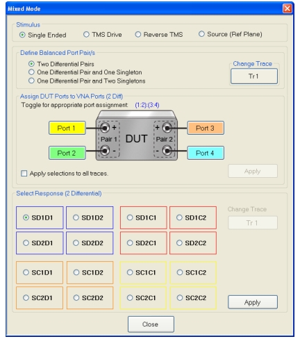
On display selection, the mixed-mode parameters will most commonly be used and the parameter selection process is the same as discussed in Multiport Measurements of this guide. This dialog is repeated in Figure: Mixed-mode Parameter Dialog here for convenience and the configuration from the TMS configuration will map by default to the response selection dialog. Although it is an unusual situation, it is allowed to use different port pairings for the mixed mode parameter definition compared to the drive configuration of TMS. The most common time this would be used would be to shift polarity within a pair to match a particular display requirement for final data. In graph legends and in the menu display, the port pair configuration is labeled as (x:y):(z:w) for pairs x-y and z-w. For the three port case, the singleton port will be outside of the parenthesis (e.g., (x:y):z). Note that the order within the pair designation denotes polarity.
Mixed-mode Parameter Dialog
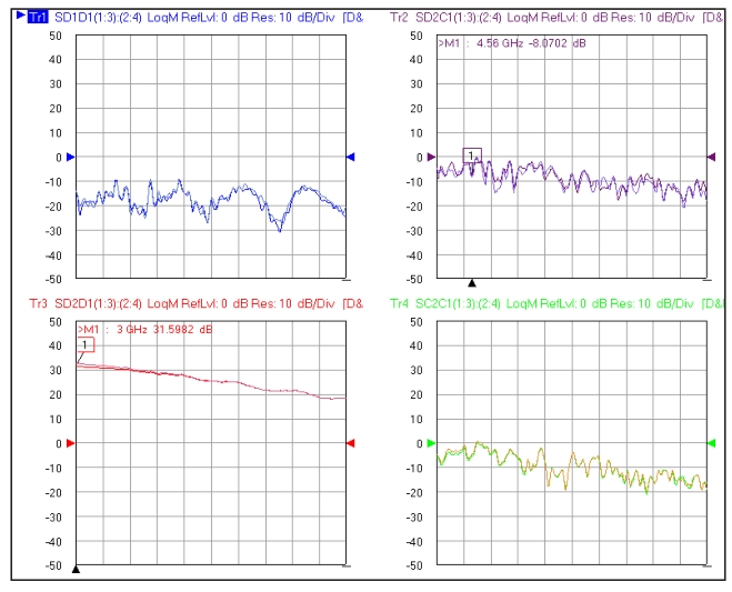
As a first example, consider a fairly linear amplifier measurement. Setups and measurements were done in both single-ended and balanced-balanced true-mode stimulus configurations. Several mixed–mode parameters of the amplifier are shown in Figure: Mixed-mode Parameters of an Amplifier. This particular amplifier had unbalanced compression mechanisms due to its topology, but was being driven at a low enough level that drive sensitivity was weak.
Mixed-mode Parameters of an Amplifier
Some mixed-mode parameters of an amplifier in both single-ended and true-mode stimulus modes are shown here at a low drive level. In this case, there was no significant difference.
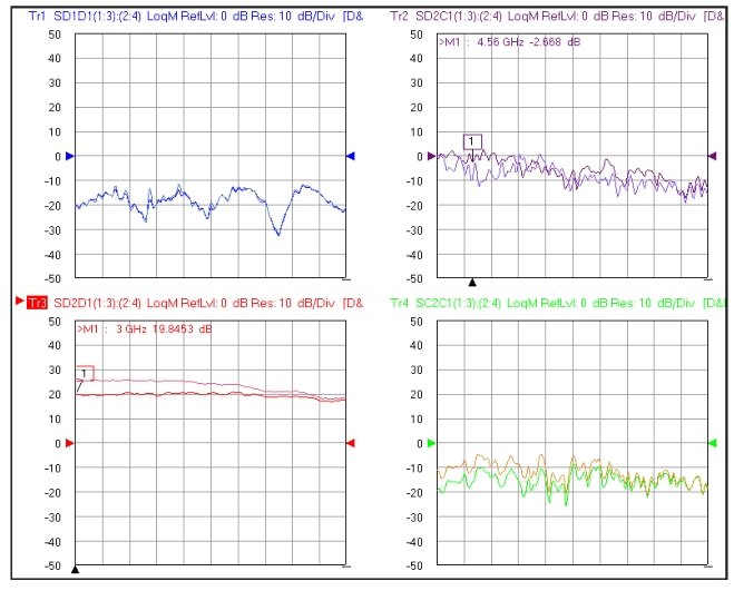
The power level was then increased to the level of several dB of compression. Since this amplifier had a very unbalanced compression response, significant differences were observed between single-ended and TMS drive. These measurements are shown in Figure: |SD2D1| Values of a Second Amplifier. Note that while the transmission parameters (including mode-conversion parameters) show differences between the drive types, the input differential match shows little change. They are not plotted here, but the mode-converting match and common mode match terms were changing rapidly.
|SD2D1| Values of a Second Amplifier
SD2D1| values of a second amplifier (for single-ended and true-mode stimulus drive) are shown here. In this case, there is a divergence at compressive drive levels
As with the 2-port version of TMS, phase and amplitude offsets are available. Some caution is required on amplitude since the default ALC calibrations are referenced to the VNA’s base two ports. Additional user power calibrations may be needed at the final reference planes to have an accurate read on absolute power. The TMS process will equalize power delivered to the DUT (in absence of an entered offset) relative to the starting value for Port 1 or Port 2 (in the 4-port case).
An important question is how do the uncertainties of the S-parameters derived with true-mode stimulus differ from those measured with single-ended stimulus? Since the error coefficients are derived from exactly the same measurements, the calibration kit-related uncertainty terms are the same. The difference lies in how the raw S-parameters from the DUT measurement are fed into the calibration. In the case of single-ended measurements, the input is obviously direct. In the true-mode stimulus case, however, raw single-ended S-parameters for use in the calibration are extracted from differential and common mode drive measurements.
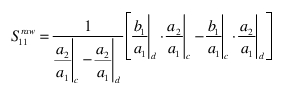
Consider the simple 2-port case, the raw S11 is found from:
Equation 26‑3.
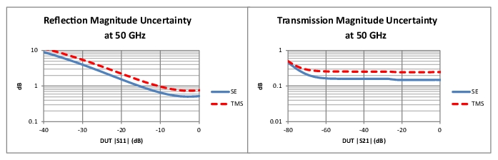
In the limiting case of perfectly in-phase (and equal amplitude) a2 and a1 for common-mode drive and perfectly out-of-phase for differential drive, this reduces to the average of b1/a1 in the two drive states. These measures are, however, subject to their own uncertainties in the stochastic terms and in the deterministic terms (while macro issues have been largely removed by the pre-measurement adjustments, the residuals still apply). Thus there is something of a compounding of uncertainties with true-mode stimulus. For the quasi-linear situations of relevance here (unbalanced compression), this uncertainty increase is small in comparison to the functional correctness, but it does suggest that true-mode stimulus will present something of a detriment to uncertainty, however modest, when linear or balanced compression measurements are called for. An example comparative uncertainty plot is in Figure: Example Comparisons of Uncertainties for Single-ended vs. True-mode Stimulus.
Example Comparisons of Uncertainties for Single-ended vs. True-mode Stimulus
Example comparisons of uncertainties for single-ended vs. true-mode stimulus in a linear S-parameter measurement are shown here. The calibrations in this case were all sliding load SOLT and the uncertainty evaluation is at 50 GHz. Drift differentials were not included.
Not included in Figure: Example Comparisons of Uncertainties for Single-ended vs. True-mode Stimulus are any differences in stability due to drift from thermal or temporal changes. Since the correction process for true mode stimulus (using Equation 26‑2. for example) is dependent on the error coefficients, any changes in those error coefficients will cause a delivered phase error along with an error in extracting the raw S-parameters. The former can be quite germane for the unbalanced nonlinear cases being discussed in this section and primarily argues for high cable quality, using as controlled an environment as possible, and performing periodic recalibrations. In the sense of the latter, this is another uncertainty adder for measurements longer after calibration time.