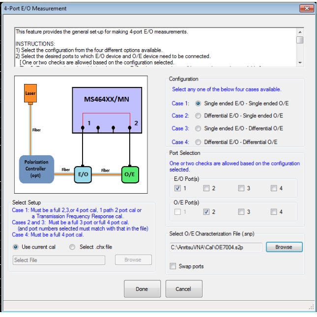
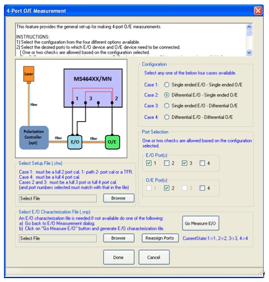
When a 4-port VNA is used, there are obviously more port permutations possible for connections but also differential or multiport O/E and E/O devices can be handled. The measurement processes are essentially the same as for the 2-port cases just discussed but there are some additional logistics to handle. For the case of solving for single-ended E/O device when used with a single-ended O/E device (Case 1 Configuration), the dialog of Figure: Case 1 Dialog—Single-ended 4-port E/O Measurements applies and the main choice is which ports are to be used.
The same rules discussed in the previous section apply on the type of calibration used (in the .chx file to be loaded or the current setup), except that the path selected (using the port checkboxes) must be covered by that calibration. In addition, full 3-port and 4-port calibrations can be used if desired (where the 3-port calibration must cover the ports being used). The characterization file in this case is again a .s2p format file with S21 as the parameter of interest.
Case 1 Configuration (Single-ended E/O—Single-ended O/E)
.
Case 1 Dialog—Single-ended 4-port E/O Measurements
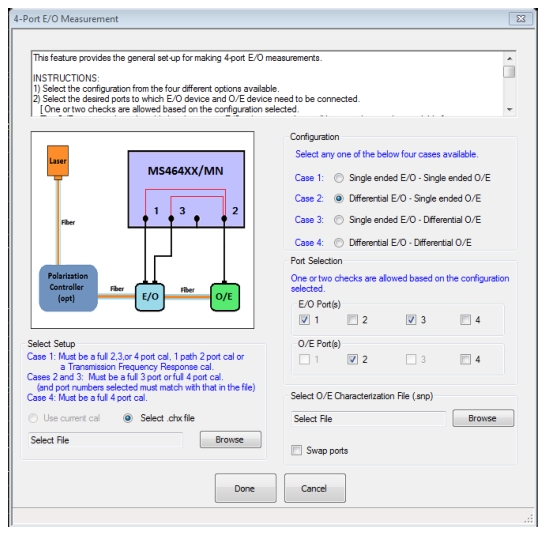
Case 2 Dialog—Variations for Different DUT Port Structures
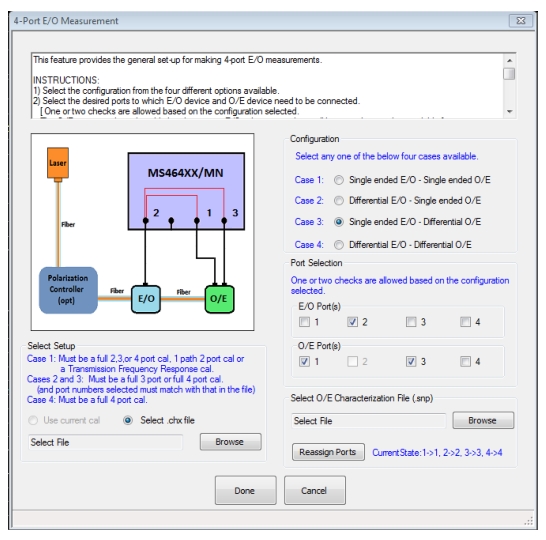
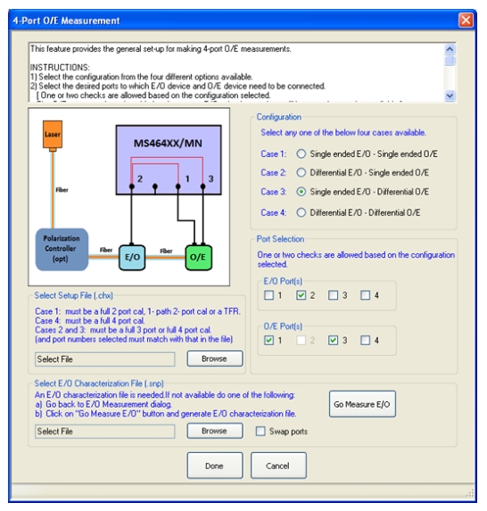
Case 3 Dialog—Variations for Different DUT Port Structures
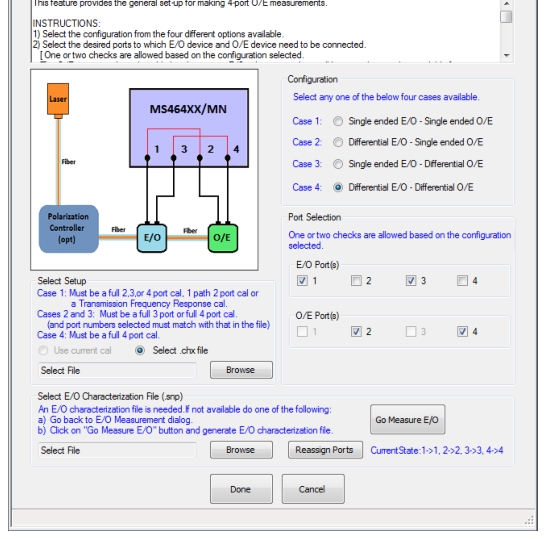
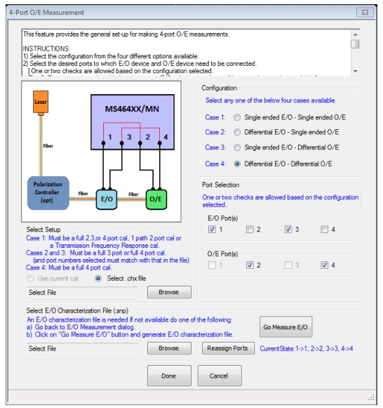
Case 4 Dialog—Variations for Different DUT Port Structures
A few things change in these other cases:
Case 2: Differential E/O—Single-ended O/E
The .chx file (or current setup, if that is used) must contain a full 3-port calibration (using the ports in question) or a full 4-port calibration of any algorithm (including hybrids).
The O/E characterization file is still of the .s2p form (S21 is the dominant parameter).
Case 3: Single-ended E/O—Differential O/E
The .chx file (or current setup, if that is used) must contain a full 3-port calibration (using the ports in question) or a full 4-port calibration of any algorithm (including hybrids).
The O/E characterization file is of a .s3p form (S21 and S23 are dominant) or a .s4p form (S21 and S43 are dominant).
The ‘reassign ports’ option is available for assigning the ports in the characterization file to match the path expectations. The current state of port reassignment is shown as a read-only field in the dialog. The default is no reassignment (1 → 1, 2 → 2, 3 → 3, 4 → 4).
Case 4: Differential E/O—Differential O/E
The .chx file (or current setup, if that is used) must contain a full 4-port calibration of any algorithm (including hybrids).
The O/E characterization file is of a .s3p form (S21 and S23 are dominant) or a .s4p form (S21 and S43 are dominant).
A Reassign Ports option is available for assigning the ports in the characterization file to match the path expectations.
In this case, there is also potential confusion as to how the DUT is exactly connected if it is “2 paths in parallel” instead is a true differential device pair. It is always assumed that the lower numbered E/O port is connected to the lower numbered O/E port. If two DUTs are being measured in parallel, make sure the port connections match this assumption.
As in the 2-port case, when one clicks Done to leave this dialog, the resident calibration will now have the O/E device de-embedded and the live measurements will reflect the behavior of the E/O device. Data and setups can be saved from this state as usual.
Caution
The .s3p and .s4p files loaded as characterization files have assumed transmission paths as detailed in the text. Use the Reassign Ports feature to make your file match those assumed paths.
For the O/E measurement case, the permutations are essentially the same and these are shown in Figure: Dialog for 4-port O/E Measurements (1 of 4). The only real difference is that case 2 and case 3 swap roles in terms of file types required as is obvious in the figure.
Dialog for 4-port O/E Measurements (1 of 4)
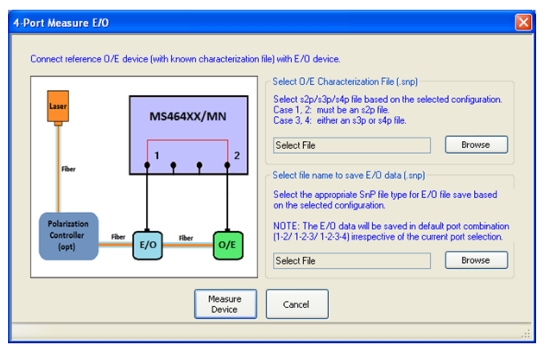
As with the 2-port O/E measurement case, there is a shortcut to go measure the E/O device to get its characterization file (assuming one has a characterized O/E device to start with such as the MN4765X). This shortcut sub-dialog is shown in Figure: Dialog for 4-port Intermediate Measurement and it must use the same case and port assignment as the parent dialog. In addition, the E/O file that is generated from this sub-dialog will follow the dominant port assignment paths that have been detailed in this section.
Dialog for 4-port Intermediate Measurement
The 4-port intermediate measurement dialog is shown here for O/E measurements when the E/O characterization file does not already exist.
4-port O/O measurements proceed analogously. The dialogs are very similar to those seen previously and will not be shown here for brevity.
• A double-path E/O device feeding a single-ended MN4765X (so this becomes case 2 under E/O measurements). The E/O device will be connected to ports 1 and 2 while the O/E device will be connected to port 3. The measurements of interest are then S31 and S32. The O/E characterization file is still of the .s2p format where S21 is the controlling parameter.
• A full three port calibration is performed using the 3654D calibration kit (SOLT) and the setup file is saved (.chx).
• The optical components are connected and powered in the appropriate order as discussed previously.
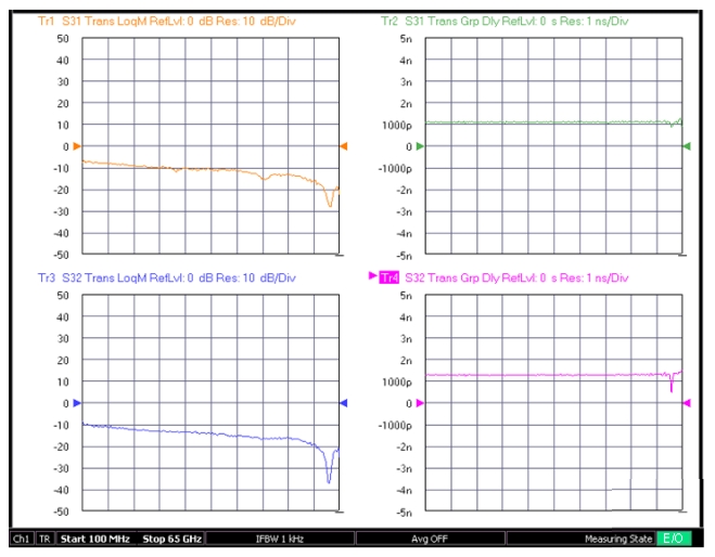
• The E/O dialog is configured as described above and, after ‘Done’ is selected, the resulting measurements are those of the E/O device. Some example possible measurements are shown in Figure: Example of what could be a Common ‘case 2’ Measurement. In this case, the device is not as symmetric as hoped (note the differences between S31 and S32) in terms of both conversion magnitude and group delay. A strong resonance is observed in both paths near 62 GHz and lower-Q resonances are seen in the S31 path at lower frequencies. This type of data could be useful in device optimization/redesign.
Example of what could be a Common ‘case 2’ Measurement
In this case, the data represents a dual-path E/O device being analyzed.