A first example shown below uses the Standard Fast CW mode and the internal buffering sub-mode. This particular measurement is of an antenna pattern where signals are available in the controller when the rotating antenna passes certain preset angles. These will be treated as sequential polling events in the below code for configuration-specific reasons but there are many other ways of performing this task. It is desired to mark the data at those points for later correlation analysis. As standard Fast CW is remote-only, this example will be presented in terms of control code. This code here is from MATLAB and other environments will do something similar although the command formatting will be different. It is assumed that the connection to the remote VNA has already been established (as object ‘obj1’) when the below commands are executed. In particular, it is important to allocate the Input and Output Buffer sizes appropriately. If transferring a large amount of data from the VNA (which we will be in this example), the Input Buffer Size (expressed in Bytes) must be able to accommodate it.
Standard Fast CW Example
% Set size of the buffer
fprintf(obj1, ':SENS:FCW:IBUF:POIN 100000’);
% Start the collection and start the rotation hardware (a user
% function call does this.
fprintf(obj1, ':SENS:FCW:DCOL CONT');
StartAntennaRotation(one_cycle);
% Mark the data during acquisition.
% The rotation is known to be slow relative to acquisition
% so a ‘while’ loop can work. When a given angle is passed in this
% setup, the bit goes high and stays high.
while Angle_90 == 0
end
% Mark the data with a 0 real (and 0 imaginary)
fprintf(obj1,':SENS:FCW:MARK 0');
while Angle_180 == 0
end
fprintf(obj1,':SENS:FCW:MARK 0');
while Angle_270 == 0
end
fprintf(obj1,':SENS:FCW:MARK 0');
% Now just wait for the internal buffer to fill up
fprintf(obj1,'WFFB');
% Get the number of points and then transfer the data from the
% The binblockread command automatically strips the header and reads
% the size. Fread can also be used but the header must be stripped
% manually. The data is read in by bytes instead of 32 bit float
% size chunks to make byte swapping simpler (LSB is first by default)
[Data, count]=binblockread(obj1,'uint8');
The variable Data would then next be processed into complex floats typically while looking for the mark variables 0+j0 that would indicate the cardinal angle positions.
Advanced Fast CW Example
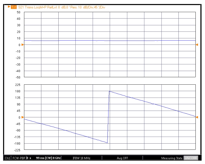
For a first Advanced Fast CW example, consider an externally synchronized measurement where a DUT has a large number of variable phase states and it is desired to step through them relatively quickly and acquire a complex S21 measurement at each step. An external control module will step the DUT state every millisecond and also send a sync pulse to the VNA (slightly delayed so it is guaranteed that the DUT is settled in time; if this was not the case, the Delay variable could be used to compensate on the VNA). Point-by-point measurements will be used since we wish to associate a measurement with each DUT state. On the Advanced Fast CW menu, the sync interval would be set for 1 ms and, since we happen to need to study 100 DUT states, the capture duration will be set to 100 ms and the number of points to 100. The measurement width was selected to be 500 μs to bring trace noise down to an improved level (the practical maximum may be on the order of 800-900 μs based on the Sync Interval). The result is shown in Figure: Advanced Fast CW Example—Point by Point along with the DUT gain although this was not as much of a focus as was the phase.
Advanced Fast CW Example—Point by Point
An example point-by-point Advanced Fast CW measurement result is shown here. A DUT was stepped through 100 phase states while the instrument received an External Synch signal to note each step.
Because the speed was not extremely high in this measurement, Standard Fast CW could have been used but the timing synchronization was simpler using Advanced Fast CW and the data processing of each measurement window could be performed by the instrument. Note that this particular measurement was performed uncalibrated and un-normalized. The user, in this case, was performing calibration off-line so the instrument was being used to collect synchronized, pre-processed raw data.
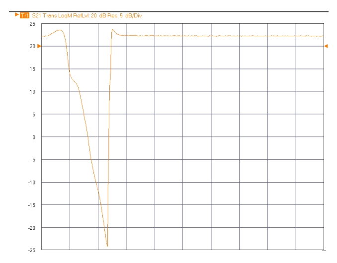
As a ‘full time record’ example, consider a module that is subject to occasional bias system transients (due to an internal overload condition). It is desired to understand how the DUT gain (at 18 GHz in this example) responds to that transient…both in terms of the duration of gain suppression and the extent of any gain overshoot on recovery or pre-shoot. The capture duration was set to 1 ms and 1000 points covering that duration were requested. The measurement width was set to 100 ns. The resulting plot is shown in Figure: Advanced Fast CW Example—Point by Point. One can see a ~ 1 dB pre-shoot and a ~1 dB overshoot in gain around the transient. The user in this case would then look to see if that transient gain change would cause issues further downstream in their system implementation. Also of interest is the very long duration of the transient (nearly 150 μs) which was unexpected since the actual bias transient at the DC source was less than half that time. The user was then investigating time constants within the bias system.
Advanced Fast CW Example—Full Time Record
A full-time record application example attempting to capture the shape of the gain effect of a bias transient on a DUT is shown here. The x-axis ranges from 0 to 1 ms (the capture duration and the stop time).
In this example, the timing resolution desired was faster than could be supported by standard Fast CW so the use of Advanced Fast CW made more sense. The UI level processing in the full time record mode also helped in speeding the analysis of the data.