For each channel defined above, from 1 (one) to 16 trace graphs (called “traces”) can be defined where each trace is a data display within a specific channel. Each trace is defined by a response parameter (such as S11), a graph type display (such as a rectilinear graph, a polar display or Smith chart), a scale, and possibly post-processing elements such as time domain and smoothing. There are four general graph types available and within each general type are multiple sub-types:
• Rectilinear single graph
• Rectilinear dual graph
• Polar plot graph
• Smith chart
Trace Data Types
The data types generated by the VNA (real, imaginary, magnitude, phase) are used in the display graph to show the possible ways in which S-Parameter data can be represented. For example, complex data, that is data in which both phase and magnitude are graphed, may be displayed in any of the following ways:
• Complex Impedance
Displayed on a Smith chart graph as impedance or as admittance
• Real and Imaginary
If simultaneous displays are required, displayed on a real and imaginary rectilinear (a Cartesian plot) graph. If only one type is required, a single rectilinear real graph or single rectilinear imaginary graph.
• Phase and Magnitude
Displayed on a single rectilinear graph, as paired rectilinear graphs, or as a polar graph
• Group Delay
Defined as the frequency span over which the phase change is computed at a given frequency point. The quantity group delay is displayed using a modified rectilinear-magnitude format. In this format, the vertical scale is in linear units of time (either ps, ns, us, or ms). With one exception, the reference value and reference line functions operate the same as they do with a normal magnitude display.
Trace Display Graphs
A separate graph can be assigned to each active channel and display area. The following available display graph types are listed in Table: Available Trace Display Types (1 of 4) below.
Available Trace Display Types (1 of 4)
Menu Name
Definition and Display Options
Y-Axis
Dependent Variable
X-Axis
Independent Variable
Measurement Applications
Rectilinear Single Graphs
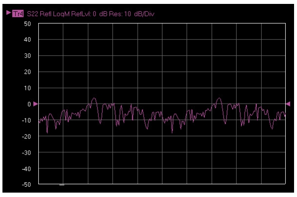
Log Mag
Log magnitude rectilinear format graph
Magnitude
Y = dB
Return loss measurement
Insertion loss measurement
Gain measurement
Linear Mag
Linear magnitude rectilinear format graph
Magnitude
Linear units
Reflection coefficient measurement
Phase
Phase rectilinear format graph
Phase displayed in range from -180 to + 180 degrees
Degrees
Linear phase deviation measurements
Imaginary
Imaginary rectilinear format graph
Imaginary part of measured complex parameter
Linear units
Real
Real rectilinear format graph
Real part of measured complex parameter
Linear units
SWR
Standing Wave Ratio rectilinear format graph
where ρ = Reflection Coefficient
Linear units
Standing wave measurements
Antenna analysis
Impedance
Impedance rectilinear format graph
Six options are:
• Real
• Imaginary
• Magnitude
• Real & Imaginary
• Inductance
• Capacitance
Polar Graphs
Linear Polar
Linear polar plot graph
The polar graph format traces are used to display one magnitude value and phase on the same chart.
Plot options:
• Lin/Phase
• Real/Imag.
Chart mode options:
• Magnitude/Phase
• Magnitude/Swap Position
Log Polar
Plot options:
• Log/Phase
• Real/Imag.
Chart mode options:
• Magnitude/Phase
• Magnitude/Swap Position
Smith Chart Graphs
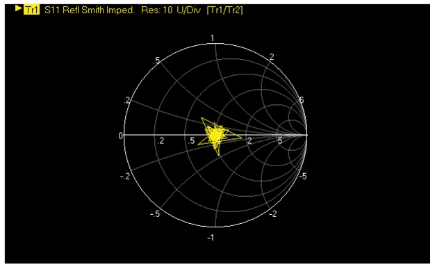
Smith (R + jX)
Smith Chart graphs with impedance (circuit resistance and reactance)
Five read out style options are available:
• Lin/Phase
• Log/Phase
• Real/Imag
• Impedance
• Impedance L/C
The impedance is the measure of a circuit’s opposition to alternating current which consists of the circuit resistance and the circuit reactance, together they determine the magnitude and phase of the impedance.
• Reflection measurements
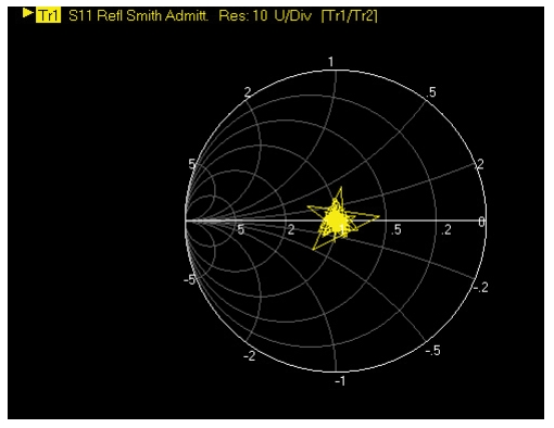
Smith (G + jB)
Smith Chart graphs showing admittance (conductance and susceptance).
Five read out style options are available:
• Lin/Phase
• Log/Phase
• Real/Imag.
• Admittance
• Admittance L/C
The admittance (Y) is the inverse of the impedance (Z) and is a measure of how easily a circuit will allow current to flow, a combination of conductance (the inverse of resistance) and the dynamic susceptance (the inverse of reactance).
Rectilinear Paired Graphs
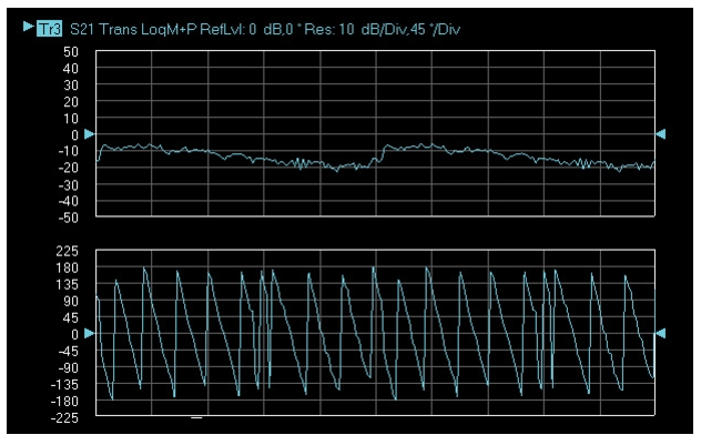
Log Magnitude and Phase
Paired graphs with Log Magnitude on top and Phase on bottom
As above
As above
Same as having one trace with a Log Magnitude display and a second trace with a Phase rectilinear display.
Linear Magnitude and Phase
Paired graphs with Linear Magnitude on top and Phase on bottom
As above
As above
Same as having one trace with a Linear Magnitude display and a second trace with a Phase rectilinear display.
Real and Imaginary
Paired graphs with Real on top and Imaginary on bottom
As above
As above
Same as having one trace with a Real rectilinear display and a second trace with an Imaginary rectilinear display.
Group Delay / Power Graphs
Group Delay
Displays the time lag through a DUT measured in ps, ns, us, or ms.
Time measured in ps, ns, us, or ms.
Frequency
Bandpass filter design
Transmission studies
Power In
Displays power in measurement through a DUT measured in dBm.
Absolute power measured in dBm.
Frequency
Efficiency
Receiver calibration
Power consumption
Power and heat dissipation
Power Out
Displays power out measurement through a DUT measured in dBm.
Absolute power measured in dBm.
Frequency
Efficiency
Receiver calibration
Power consumption
Power and heat dissipation
Each graph type is described in greater detail below with sample graphs, and explanation of supporting trace displays.
Trace Labels
Each trace (i.e. each graph display) is labeled with information such as its trace number, the graph type, scaling, reference delay, and S-parameter associated with that trace. Depending on the trace settings and the graph type, other information may be displayed.
The general format of trace label consists of the following parameters and their associated abbreviations appearing from left to right in the trace label. Some parameters may not appear depending on the instrument settings.
• Trace Number
• Trace Memory Statistics
• Inter-Trace Math Factor
• Measurement Type
• Graph Type
• Reference Level
• Resolution Units
• Conversion Factor
• Time Domain
Trace labels can be customized by the user in the DISPLAY SETUP menu and toggled on or off as an alternate trace name.
• MAIN |Display | DISPLAY | Display Area Setup | DISPLAY SETUP | Edit Alternative Trace Name | EDIT ALTERNATE TRACE NAME dialog box
Trace Label Abbreviations
The trace label abbreviations are described in the three tables below:
Trace Labels - Trace Number, Measurement Type (1 of 2)
Abbreviation
Definition
Description
Trace Number Abbreviation
Tr#
Trace number
Trace 1 through Trace 16.
Measurement Type Abbreviations
S11 Refl
S11 Port 1 forward reflection
S-parameters are selected on the RESPONSE menu.
S12 Trans
S12 Port 1 reverse transmission
S21 Trans
S21 Port 2 forward transmission
S22 Refl
S22 Port 2 reverse reflection
IM(n)
The IMD product in dBc terms
Product level relative to the main tone level.
n = the product order (can be 2,3,5,7 or 9)
OIP(n)
Output Referred Nth order Intercept point
Calculated intersection of the main tone power and product power based on the measurement at one power level.
n= the product order (can be 2,3,5,7 or 9)
Pwr(n)
Power of IMD main tone or Nth order IMD products
Tone power: represents the absolute power of a main tone (n=1) or of a product (n = 2,3,5,7, or 9)
Asym(n)
IMD Asymmetry
Difference between upper and lower amplitudes of a given order (including order 1 for main tones).
n = the tone or product order (can be 1,2,3,5,7 or 9)
b1/1/Pm
or
b2/1/Pm
When in ordinary multiple source (not an IMD mode), a power sweep of an IMD main tone or of a product can be orchestrated. The displayed response is a standard unratioed wave variable (usually b1/1 or b2/1).
m = the driving port (can be arbitrary if both sources are driving in an Option 31 equipped system)
[x] Noise Figure
Noise Figure response of [x]
x can denote B1 receiver path, B2 receiver path, Differential mode [Diff] or Common mode [Comm]
[x] Noise Temperature
Noise Temperature of [x]
x can denote B1 receiver path, B2 receiver path, Differential mode [Diff] or Common mode [Comm]
[x] Noise Power
Noise Power of [x]
x can denote B1 receiver path, B2 receiver path, Differential mode [Diff] or Common mode [Comm]
[x] Available Gain
Available Gain of DUT if output saw conjugate match, based on loaded S-parameters (in Noise Figure application)
x can denote B1 receiver path, B2 receiver path, Differential mode [Diff] or Common mode [Comm]
[x] Insertion Gain
Insertion Gain of DUT, based on loaded S-parameters (in Noise Figure application)
x can denote B1 receiver path, B2 receiver path, Differential mode [Diff] or Common mode [Comm]
Gain Compression
--
If Gain Compression is off, the @CP trace label does not appear after the Measurement Type.
For example, Tr3 S21 Trans LogM
@CP
If Gain Compression is on, the @CP (at Compression Point) appears after the Measurement Type.
For example, Tr3 S21@CP Trans LogM
NN / DD | Port #
NN is user-defined numerator value.
DD is user-defined denominator value.
Port number
User-defined numerator, denominator, and driver port are selected on the RESPONSE | User-defined | USER-DEFINED menu.
Numerator and denominator options are A1, B1, A2, B2, or 1.
Port number selection options are Port 1 or Port 2.
Ext.In [DC1 | P#]
External Analog Input 1
Driver Port number
User-defined External Analog Input 1 port is selected on the RESPONSE | Ext. Analog In 1 | EXT. ANALOG IN 1 menu.
Port number selection options are Port 1 or Port 2.
Ext.In [DC2 | P#]
External Analog Input 2
Driver Port number
User-defined External Analog Input 2 port is selected on the RESPONSE | Ext. Analog In 2 | EXT. ANALOG IN 2 menu.
Port number selection options are Port 1 or Port 2.
Rectilinear Single Graph
Trace Labels - Abbreviation, Type and Name, Reference Level Units, Resolution Units (1 of 2)
Graph Abbreviation
Graph Name and Type
Reference Level (RefLvl)
Resolution Units (Res)
Rectilinear Single Graph
LogM
Log Mag (Log Magnitude) rectilinear
dB
dB/Div
LinM
Linear Mag (Linear Magnitude) rectilinear
U
U/Div
Phase
Phase rectilinear with units in degrees (º)
º
º/Div
Real
Real rectilinear
U
U/Div
Imag
Imaginary rectilinear
U
U/Div
SWR
SWR rectilinear
U
U/Div
Imped Real
Impedance Real rectilinear with units in Ohms (Ω)
Ω
Ω/Div
Imped Imag
Impedance Imaginary rectilinear
Ω
Ω/Div
Imped Mag
Impedance Magnitude rectilinear
Ω
Ω/Div
Imped R + I
Impedance Real and Imaginary rectilinear. A rectilinear paired graph.
Ω
Ω/Div
Capacitance
Capacitance rectilinear
F
fF/Div
Inductance
Inductance rectilinear
H
pH/Div
Smith Charts with Impedance or Admittance
Smith Imped
The display can be one of four possible Smith Chart with impedance displays:
• Smith (R+jX) Linear/Phase Smith Chart
• Smith (R+jX) Log/Phase Smith Chart
• Smith (R+jX) Real/Imaginary Smith Chart
• Smith (R+jX) Impedance Smith Chart
• Smith (R+jX) L/C Smith Chart
—
U/Div
Smith Admitt
The display can be one of four possible Smith Chart with admittance displays:
• Smith (G+jB) Linear Phase Smith Chart
• Smith (G+jB) Log Phase Smith Chart
• Smith (G+jB) Real/Imaginary Smith Chart
• Smith (G+jB) Admittance Smith Chart
• Smith (G+jB) L/C Smith Chart
—
U/Div
Polar Graphs
Lin Pol
Linear Polar, Linear/Phase polar
U
U/Div
Lin Pol, RI
Linear Polar, Real/Imaginary polar
U
U/Div
Log Pol
Log Polar, Log/Phase polar
dB
dB/Div
Log Pol, RI
Log Polar, Real/Imaginary polar
dB
dB/Div
Rectilinear Paired Graphs
LogM + P
Log Magnitude and Phase rectilinear paired graphs.
dB, º
dB/Div, º/Div
LinM + P
Linear Magnitude and Phase rectilinear paired graphs
If Conversion is on, the conversion factor is appended to the right of the trace annotation.
[Zr]
Z: Reflection
[Zt]
Z: Transmission
[Yr]
Y: Reflection
[Yt]
Y: Transmission
[1/S]
1/S
Inter-Trace Math (ITM) Abbreviations
—
If Inter-trace math is off, no abbreviation appears.
[ITM]
If Inter-Trace Math is on, the math factor abbreviation (described below) is appended to the right of the trace annotation.
[Con, ITM]
If Conversion (above) is on, the Inter-Trace Math abbreviation appears to its right, separated by a comma.
Tr
Trace number
Inter-trace math can utilize any trace number that is currently defined.
[Tr + Tr]
Inter-trace math addition.
The trace number assigned to Operand 1 plus value of the trace number assigned to Operand 2.
[Tr - Tr]
Inter-trace math subtraction.
The trace number assigned to Operand 1 minus value of the trace number assigned to Operand 2.
[Tr * Tr]
Inter-trace math multiplication.
The trace number assigned to Operand 1 times value of the trace number assigned to Operand 2.
[Tr / Tr]
Inter-trace math division.
The trace number assigned to Operand 1 divided by the value of the trace number assigned to Operand 2.
[EQN]
Equation Editor
If using Equation Editor, [EQN] notation will show.
A rectilinear graph is a display of a Cartesian coordinate system or plane consisting of an X-axis and a Y-axis. The X-axis displays the independent variable (such as frequency or time) and the Y-axis displays the dependent value.
As above, but paired with a phase rectilinear graph below. Useful to save a channel, or provide immediate comparison with a function value and its phase.
The power reflected from a DUT has both magnitude and phase because the impedance of the device has both a resistive and a reactive term of the form r+jx. The r is referred to as the real or resistive term, while the x is called the imaginary or reactive term. The j, sometimes denoted as i, is an imaginary number. It is the square root of –1. If x is positive, the impedance is inductive, if x is negative the impedance is capacitive. The size and polarity of the reactive component x is important in impedance matching. The best match to a complex impedance is the complex conjugate which means an impedance with the same value of r and x, but with x of opposite polarity. This term is best analyzed using a Smith Chart, which is a plot of r and x.
To display all the information on a single S-parameter requires one or two traces, depending upon the desired format. A very common requirement is to view forward reflection on a Smith Chart (one trace) while observing forward transmission.
Smith Chart with Impedance (Circuit Resistance and Reactance)
The Smith Chart with impedance (Smith R + ex) has four display options:
• Lin/Phase
• Log/Phase
• Real/Imag.
• Impedance
• Impedance L/C
The impedance is the measure of a circuit’s opposition to alternating current which consists of the circuit resistance and the circuit reactance, together they determine the magnitude and phase of the impedance.
Smith Chart with Impedance (R+jX)
Smith Chart with Admittance (Conductance and Susceptance)
The admittance (Y) is the inverse of the impedance (Z) and is a measure of how easily a circuit will allow current to flow, a combination of conductance (the inverse of resistance) and the dynamic susceptance (the inverse of reactance). Smith Chart graph display showing admittance (conductance and susceptance) has four read out style options are available:
• Lin/Phase
• Log/Phase
• Real/Imag
• Admittance
• Admittance L/C
Smith Chart with Admittance (G+jB)
Polar Graphs
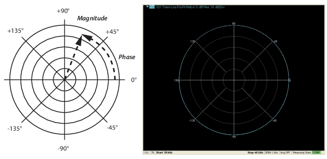
A polar graph represents a two-dimensional coordinate system where each point is determined by an angle and a distance. The polar coordinate system is especially useful in situations where the relationship between two points is most easily expressed in terms of angles and distance such as in phase relationships in antenna and feedline design. The magnitude parameter can use either a linear or log scale. As the coordinate system is two-dimensional, each point is determined by two polar coordinates: the radial coordinate (distance from the center) and the angular coordinate (degrees counterclockwise from the right edge). Polar displays are used for transmission measurements, especially for cascaded devices in series. The transmission result is the addition of the phase and log magnitude (dB) information in the polar display of each device.
Log Polar Diagram and Trace Graph Example
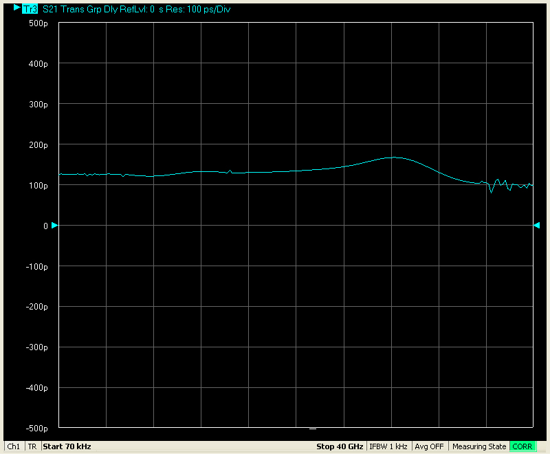
Group Delay Graphs
The quantity group delay is displayed using a modified rectilinear-magnitude format. In this format the vertical scale is in linear units of time (ps, ns, us, ms). With one exception, the reference value and reference line functions operate the same as they do with a normal magnitude display. The exception is that they appear in units of time instead of magnitude.
Group Delay Trace Graph Example
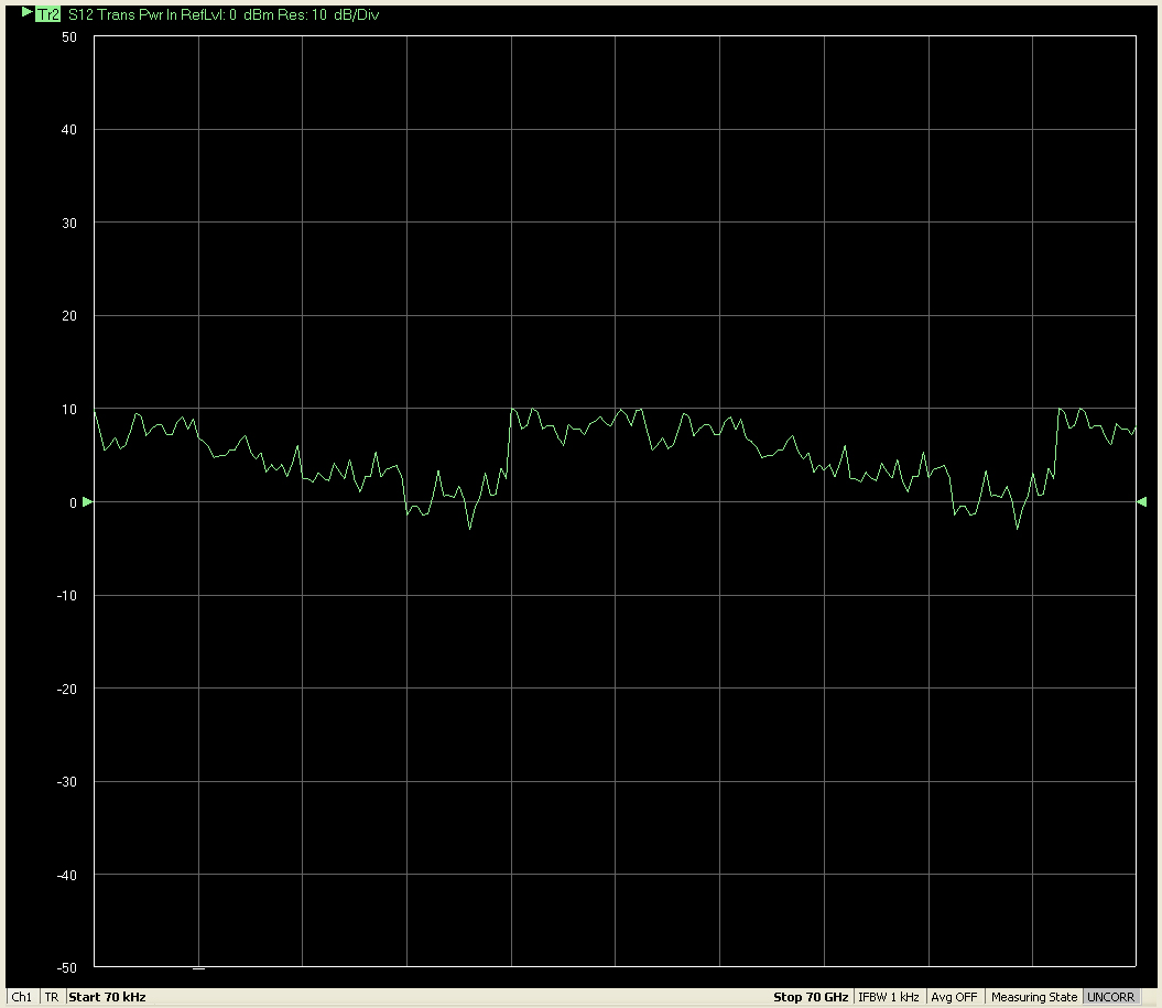
Power Graphs
Power In Trace Graph Example
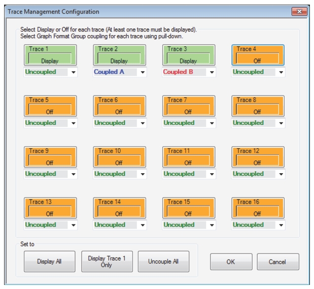
Trace Management
The Trace Management dialog box can be used to control the visibility of a trace on the UI. Individual traces can be set to 'Display' or can be turned 'Off'.
Traces can be left uncoupled or can be assigned to one of two coupled groups (A and B). Within a coupled group, the graph types and scales are forced to be the same. If a new member is added to a group, it is coerced to the format of the others in the group, and changing format of any member of the group will change the format of all members of the group.
The grouping process facilitates dual-Y-axis displays when multiple traces are overlaid. If members of A and B groups are overlaid and a member of either group is the active trace, both Y-axes will be displayed (with A and B annotations). If an uncoupled trace is active in such an overlay situation, only the Y-axis for that trace will be visible.