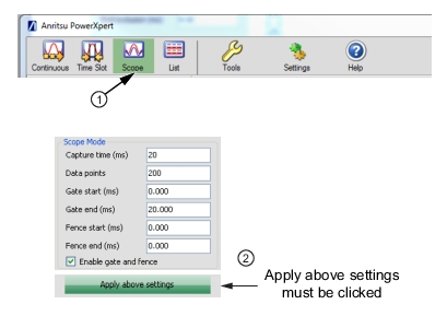
Scope mode is available with power sensor models MA24x08A, MA24x18A, MA24126A and MA243x0A. In Scope mode, the sensor acts similarly to an oscilloscope in that it can be used to measure power as a function of time. A Scope mode display is shown in Figure: Scope Mode Graphical Display Area.
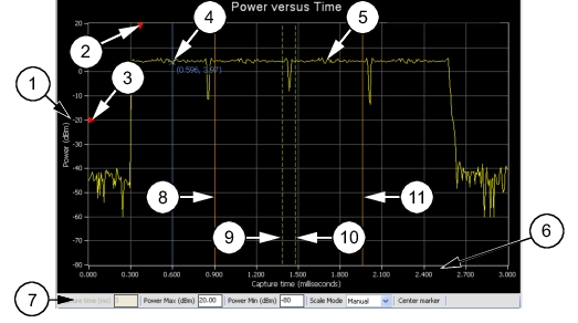
Scope Mode Graphical Display Area
Index
Description
1
The vertical scale displays the power level in dBm.
2
Trigger Delay Time showing the current trigger delay position. The trigger delay is set in the Trigger Settings area. See Trigger Settings.
3
Trigger Level Marker showing the current trigger level position. The trigger level is set in the Trigger Settings area. See Trigger Settings.
4
Marker showing as a vertical blue line with an x on the marker point and numerical values for the time (ms) and power level (dBm). The marker is available for reading power at an instant of time. It can be dragged with the mouse and can be centered in the display via the Center marker button.
5
Graphical trace display showing the power level as a function of time.
6
The horizontal scale displays the total capture time (in milliseconds) and may be increased or decreased from the Scope mode settings area.
7
Graticule Settings:
Capture Time: Displays the current capture time setting. This setting is changed in the Scope Mode settings window. Power Max (dBm): Sets the upper power level for the vertical scale. Power Min (dBm): Sets the lower power level for the vertical scale.
• Power Max (dBm) and Power Min (dBm) settings are not available when set to Automatic.
Scale Mode: Sets the vertical scaling to Automatic or Manual.
Changes to these settings are applied by pressing the Enter key.
There are two parameters needed to define the Scope mode operation:
• Capture time
• Number of data points.
The sensor first waits for a trigger. Upon receiving a trigger, the sensor starts collecting data at its sample rate for the duration of the capture time. This will typically result in a number of samples that exceed the number of displayed data points. In this case, individual samples are averaged together to display the requested number of data points.
Capture Time
The Capture Time represents the time displayed on the screen at any one time. If a positive delay is specified for the trigger delay item, the capture time will commence once the specified delay has been reached.
Data Points
Scope mode can be used to look at very fine structures of a signal. When using marker, gate, and fence, the power of any specific time can be accurately measured. To better observe these fine signal structures, a graph capture time can be reduced to get better resolution. However, as capture time shrinks, the time intervals between data points on the graph also decrease. The capture time can continue to shrink until it approaches the absolute resolution limit.
The sampling rate of the MA241xxA series power sensors is approximately 131 kS/s, or 7.6 µs per sample. The sampling rate of the MA242x8A and MA243x0A series power sensors is approximately 140.056 kS/s, or 7.14 µs per sample. When the capture time divided by the number of points is at 7 µs, the resolution has reached its maximum. Any more reduction in capture time must be accompanied by a reduction in the number of data points such that:
(capture time)/(data point) > 7 µs
For example, in case of a MA24118A with 20 ms of capture time, there are 2860 samples. If there were 10 data points, then each data point consists of an average of 286 samples. The number of data points should not be less than the total number of samples. For a given capture time, the lower the number of data points the more samples that are averaged per point, thus the lower the trace noise.
When there is a large number of points in a graph, the points are plotted at the beginning of the given time interval. For example, if a graph has a capture time of 100 ms and data points of 1000, then the first time interval is from time 0 µs to 100 µs (100 ms/1000). The power measured during this time interval is plotted as a point at time 0 µs. Subsequent intervals are plotted the same way until time interval 1000, where data is plotted as a point at time 99.9 ms. When there are many data points in a graph, not having a point at exactly 100 ms is not noticeable. However, when there are fewer points, then the graph seems incomplete (missing the last data point). One may perceive this as a time inaccuracy if not aware of how the graph is plotted.
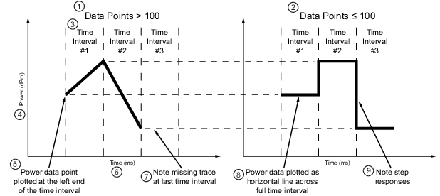
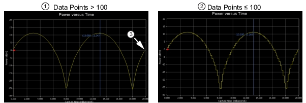
When the number of points reaches 100, PowerXpert implements a different type of graphing that is more technically correct. Instead of plotting each time interval as a point, time intervals are plotted as a horizontal line between the start and the end of the time interval. For example, if a graph has a capture time of 1 ms and data points of 100, then the first time interval will be from 0 μs to 10 μs (1 ms/100). The power measured during this time interval is a horizontal line representing the measured power plotted between time 0 μs to 1 μs. Subsequent time intervals are plotted the same way until time interval 100, where a horizontal line is plotted between time 990 μs and 1 ms. See Figure: Data Point Plot Difference Description. The resulting power graph will look different as seen in Figure: Data Points Plot Differences.
Data Point Plot Difference Description
Index
Description
1
Data Points > 100
2
Data Points ≤ 100
3
Time Intervals (#1, #2, #3)
4
Power (dBm)
5
Power data point plotted at the left end of the time interval
6
Time (ms)
7
Note missing trace at last time interval
8
Power data plotted as horizontal line across full time interval
9
Note step responses
Data Points Plot Differences
Index
Description
1
Data Points >100
2
Data Points ≤100
3
Note the missing trace at the last time interval in the plot on the left.
Gate and Fence
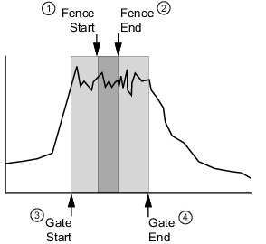
The Gate and Fence feature enables measurement of the desired portion of the waveform. A Gate is a specification for extracting an averaged power reading measurement between two defined points on a pulsed waveform. A fence must be set up within the boundaries of a gate, unless the fence is disabled by setting the Fence start and end to zero, or to the same value. All data sampled between the fence start and end positions are excluded from the average power calculations for the gate. This is useful for purposes such as excluding a training sequence from an EDGE measurement.
Gate and Fence Mode Settings
Index
Description
1
Fence Start
2
Fence End
3
Gate Start
4
Gate End
Checking the Enable gate and fence box enables the feature in PowerXpert. All of the gate and fence settings are relative to the triggering event (start of capture). The fence must reside entirely within the gate, unless the fence is disabled by setting the Fence start and Fence end to zero. The gate and fence start and end points can be dragged by the mouse or directly entered: (the Apply above settings button must be clicked to enable the changes to the gate and fence parameters, even when dragging them with the mouse).
Certain restrictions and conditions apply when setting up gating and fence settings as listed below:
• Gate start cannot be negative and it cannot exceed the capture time.
• Gate end value cannot be less than gate start and cannot exceed the capture time.
• Fence start should be between Gate start and Gate end.
• Fence end should be between Fence start and Gate end.
• If the Fence start and Fence end values are the same, then the fence is disabled.
• Fence is disabled if both fence start and fence end are set to zero.
• The Fence start and Fence end positions cannot be set outside of the area defined by the Gate start and Gate end positions.
• The Gate start and Gate end points are included in the measurement.
• The Fence start and Fence end points are excluded from the measurement and have priority over the Gate start and Gate end points if they coincide.