This chapter describes calibration procedures using the SOLT/SOLR calibration algorithms. One of the more common calibration algorithms is based on Short-Open-Load-Thru. This is a defined-standards calibration meaning the behavior of all of the components is specified in advance via data or models.
Since the behaviors of all standards are known, by measuring them with the VNA we can define all of the error terms. The load behavior largely sets the directivity terms, the short and open together largely determine source match and reflection tracking and the thru largely determines transmission tracking and load match.
Related Chapters
The following contains content related to SOLT/SOLR Calibration:
Shorts can be defined by a model consisting of a transmission line length and a frequency-dependent inductance or with a .s1p file describing the reflection coefficient.
Opens
Opens can be defined by a model consisting of a transmission line length and a frequency-dependent capacitance or with a .s1p file describing the reflection coefficient.
Loads
Loads can be defined by a model consisting of a transmission line length, a shunt capacitance, a resistance and a series inductance or with a .s1p file describing the reflection coefficient.
Note that a sliding load can be used in lieu of a fixed load. The sliding load is based on a sliding termination embedded in an airline and the transmission line properties of that airline are used to deduce a more nearly perfect synthetic load. Because of the transmission line dependence, a fixed load is also needed at low frequencies (below 4 GHz for V connectors (shorter sliding load) and below 2 GHz for others).
The .s1p-based load definition can perform as well as a sliding load in most cases and will almost always outperform a simpler modeled definition.
Thru
Modeled as a transmission line length with some frequency-dependent loss. A root-f frequency dependence of that loss is assumed. A .s2p-defined thru is also possible where loss and mismatch are used. Interpolation and extrapolation of the .s2p data will be used to complete the calibration. A 'characterize thru' option is also available to help generate such an .s2p file based on a network extraction method (Type B, see Adapter Removal Calibrations and Network Extraction of this guide for more information).
Reciprocal
The thru can sometimes be replaced by a unknown but reciprocal network (like an adapter or a fixture) when an actual thru connection is not practical. The accuracy will be somewhat less than if an actual thru could have been used but will be better than assuming a poor thru is a good one.
Notes on .s1p Cal Kit Definitions:
• These are provided with some Anritsu calibration kits when Option 3 or Option 4 is ordered. The data files shipped with those calibration cal kits also include a .lst file that allows loading of .s1p files for all calibration kit components simultaneously.
• The user can also generate their own .s1p files for calibration kit components based on measurement, electromagnetic modeling or some other means. If based on measurement, it is recommended that a higher accuracy calibration form the basis of the characterization (e.g., LRL based on beadless airlines for coaxial situations).
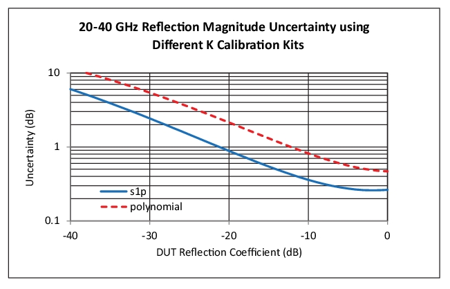
• The use of a .s1p-based calibration can substantially improve uncertainties in measurement. As an example, consider the use of an Anritsu 3652A K calibration kit to perform a reflection measurement between 20 and 40 GHz. The uncertainties are plotted below both using the old polynomial model and using the .s1p definition available with Option 3 or Option 4 on that cal kit. Consult the MS464xB Technical Data Sheet (11410-00611) for a more complete comparison.
Comparison of Reflection Magnitude Uncertainty with s1p vs. Polynomial Definitions
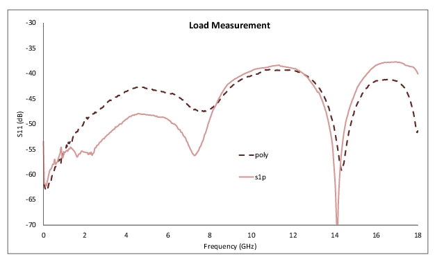
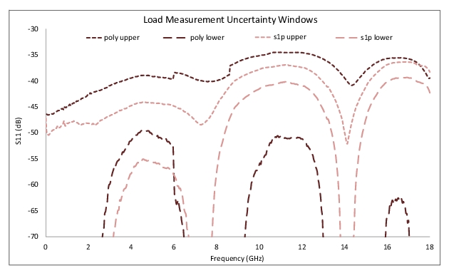
The results can get more confusing when measuring very small reflections since the uncertainties are becoming proportionately larger in both cases. Consider the measurement of a load (not used during calibration). The measurements using two different calibration kit definitions are shown in Figure: Load Measurement Comparing Two Different Calibration Kit Definitions (Polynomial vs. s1p) below along with the uncertainties for those measurements.
Load Measurement Comparing Two Different Calibration Kit Definitions (Polynomial vs. s1p)
Note that the absolute return losses differ considerably, particularly at low frequencies, but because the reflections are so low, these differences are within the uncertainties. Note also (very clear at higher reflection levels) how much narrower the uncertainty windows are for the .s1p-based calibration. Below about –50 dB reflection coefficients, the uncertainties are quite high for both methods.