De-embedding is covered in detail in Calibration and Measurement Enhancements but since the generation of files for some de-embedding exercises is so closely tied to adapter removal; it will be briefly discussed now. De-embedding is the removal of the effects of a network from a set of data. This network could represent an adapter or fixture, among other things. To perform the de-embedding, the parameters of this network must be known. While there are many methods of deriving these parameters (including simulation), measurement in some way is often preferred. Because of the complex and incompatible media that may be involved, techniques using multiple calibrations (in different connectors or different media) or techniques using a pair of adapters/fixtures back-to-back are sometimes employed.
Two full 2-Port calibrations are performed; one each with the adapter/fixture attached to one port, then the other. A single S2P file describing the adapter/fixture is generated. This is directly the method of adapter removal except the parameter file is generated explicitly rather than the calibration being directly modified. Refer to Type A Network Extraction.
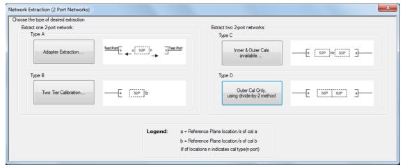
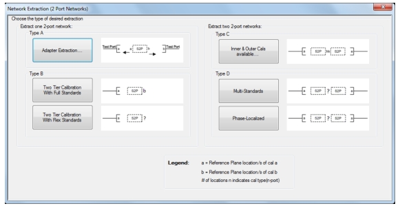
Type B—Two Tier Calibration With Full Standards
A two tier calibration, sometimes called 1-Port de-embedding or the Bauer-Penfield technique. Here a one port cal is performed, and then additional standards are measured with the adapter/fixture in place. A thru connection is not required, which can be convenient in many cases, and a single .s2p file is generated. In the full standards case (an entire second calibration is required at the end of the adapter/fixture), the calculation is similar to Type A, except the outer match is handled differently. Refer to Type B Network Extraction.
Type B—Two Tier Calibration With Flex Standards
Algorithmically, this is similar to the full standards case, but a different, or incomplete, calibration may be performed at the fixture output plane. Additional assumptions are made as the standards count dropped (e.g., with one standard, fixture match is neglected).
Type C—Inner and Outer Cals Available
This is the network extraction method available in earlier generations of Anritsu VNAs where full 2-port calibrations are performed at the outer plane (often coaxial or waveguide) and at the inner plane (often a fixtured environment). Two S2P files are generated in this case. Refer to Type C Network Extraction.
Type D—Outer Cals Using the Divide-By-Two Method (Multi-Standards)
This simplified method is used when standards at the inner plane are difficult to create (as in a complicated fixture structure). Two adapter/fixture “halves” are connected back-to-back and/or with some standards between them and the combination measured using a single outer cal. Assuming the interconnect between the two halves is well-matched and the two halves are identical, S-parameters can be extracted. At least one thru interconnect between halves is needed and an additional (different length) interconnect can be used or high reflection standards can be used at the inner plane. If only one interconnect is used, inner plane match is assumed perfect. Additional information is obtained and accuracy generally improves as more standards are added. Two S2P files are generated. Refer to Type D Network Extraction—Multi Standards (with Option 21).
Type D—Phase Localized
A variation of type D makes use of knowledge of fixture length (through user entry or model fitting) to better localize mismatch and enable a more accurate extraction if the fixture is electrically long enough. Refer to Type D Network Extraction—Phase Localized (with Option 21).
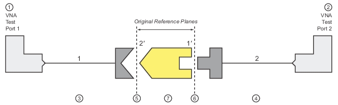
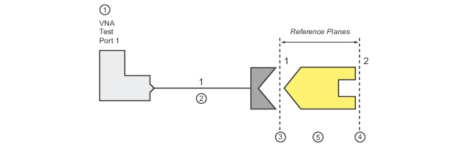
As discussed above, the Type A extraction uses exactly the same procedure and algorithm as adapter removal. Instead of directly modifying the calibration to remove the effects of the adapter/fixture, however, the S-parameters of the adapter/fixture are exported to an S2P file for later de-embedding or other uses. The reference plane diagram is repeated below for convenience. Two full 2-Port calibrations are required, one with the adapter on Port 1 (so the cal is between 1’ and 2) and one with the adapted on Port 2 (so the cal is between 1 and 2’).
Adapter Removal Block Diagram
1. Test Port 1
2. Test Port 2
3. Port 1 Test Cable
4. Port 2 Test Cable
5. Original Reference Plane 2’, when adapter is connected to Port 2 Test Cable
6. Original Reference Plane 1’, when adapter is connected to Port 1 Test Cable
7. Adapter to be calibrated
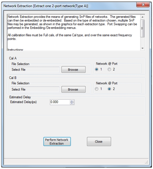
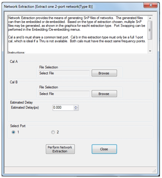
The calibrations are performed and then the setups saved typically as an active channel CHX file type. The extraction dialog is shown below where these files are retrieved to perform the process. After “Perform Extraction” is selected, a new dialog will appear asking for the file name where the S2P data should be saved.
As with adapter removal, a few caveats apply
• The two calibration files must have the same frequency lists (i.e., same frequency range and same number of points).
• The cal algorithms and media types may be different but they must both be full 2-Port cals
• The adapter is assumed to be reciprocal (S12 = S21).
NETWORK EXTRACTION Dialog Box—Extract One 2-Port Network—Type A—2-Port VNAs
Type B Network Extraction
The Type B extraction is a simplification of Type A in that it only requires one port standards. There are two variations of Type B: full standards and flex standards. Both variants can be useful if a thru connect is difficult to implement because of adapter/fixture configuration issues. Below are descriptions of the two versions:
Full Standards: Requires three reflect standards (a full one-port calibration) at the far end of the fixture arm. This completely solves the reciprocal error box describing the fixture but does require three known standards.
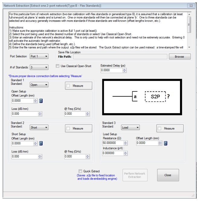
Flex Standards:This allows 1, 2 or 3 reflection standards to be used at the far end of the fixture arm for cases when a variety of different standards may be available. The three-standard case is simply a generalization of the ‘full calibration’ case where a variety of different standards can be easily tried if independent (e.g., 2 offset opens and a load, 2 offset shorts and an offset open, etc.). The one and two standards cases make assumptions about the fixture (partial information techniques) for cases when few known standards are available. An additional option will be required (Option 21) for this choice to be available.
Type B Network Extraction—Full Standards
The full calibration algorithm has a long history and is covered in the literature extensively (for example, R. Bauer and P. Penfield, “De-embedding and unterminating,” IEEE Trans. Micr. Theory Tech., vol. 22, pp.282-288, Mar. 1974.). As suggested by the figure below, a calibration is performed at Plane 1 (often a coaxial or waveguide calibration) and a second calibration is performed at Plane 2 (could also be coaxial or waveguide in the case of an adapter or could be more complicated in the case of a fixture).
Network Extraction Type B Reference Planes
1. Test Port 1
2. Port 1 Test Cable
3. Original Reference Plane for Port 1
4. Second Reference Plane at end of Adapter DUT
5. Adapter DUT
As before, the cals are performed and the setups saved, typically as an active channel CHX file type. The cal files are retrieved using the dialog shown below.
NETWORK EXTRACTION Dialog Box—Extract One 2-Port Network—Type B—With Full Standards
After Perform Network Extraction is selected, another dialog appears asking for the file name where the resulting S2P data should be saved. Different cal algorithms and media types may be selected but at least Cal B must be 1-Port only. Cal A can be a full 2-port cal or a double 1-Port cal (this way it is known how to compute the extraction). As with Type A, the adapter/fixture is assumed to be reciprocal and the frequency lists must be the same.
The results obtained with Type B may be somewhat different from those obtained with Type A since the algorithms are not the same. The main differences will be with respect to outboard match (at Plane 2 in Figure: Network Extraction Type B Reference Planes above). In Type A, this match is determined with a full reflectometer solve while in Type B, it is determined with a source-match like extraction on the error X of the second cal. As a result, the Type B extraction of this match will be somewhat more sensitive to cal quality than will Type A (particularly with regard to the source match-determining cal components: O and S in OSL or the two shorts in SSL). The trade-off is simplicity and, in some cases, practicality.
Type B Network Extraction—Flex Standards (with Option 21)
There are a number of cases where it is not practical to perform a conventional one-port calibration at the far end of the fixture arm. An unusual set of three standards may be all that is available or only one or two reasonably-well-known standards exist. The ‘flex standards’ variant handles these cases. As with ‘full standards’ the user will select the port in question, an estimate of the length of the arm (and use 0 for an automatic estimate) and where to save the .s2p file for the fixture arm. Also as in the ‘full standards’ case, the fixture will be assumed to be reciprocal but not necessarily symmetric. In this variant, the user must also select the number of standards as shown in the below dialog.
NETWORK EXTRACTION Dialog Box—Extract One 2-Port Network—Type B—Flex Standards Variant
When using one standard, only the insertion loss and phase of the fixture arm will be solved for and the match will be assumed to be perfect. If the fixture is well-matched anyway (e.g. the return loss is >15 dB and no deep return loss DUTs need to be measured), this can be a good choice. If only one defined standard is available (e.g., only an open-ended fixture is available), this may be the only choice. Obviously there will be some added uncertainty as fixture mismatch increases. Almost always a high-reflect standard (e.g., open or short) is used for this method.
When using two standards, the mismatch of the fixture arm is assumed to be symmetric but not perfect. If the fixture loss is low, this can be a reasonable approach and is particularly popular in on-wafer applications (also termed an open-short de-embedding method). Most commonly, two high reflect standards are used for this method but a higher return loss device can be substituted to tilt the uncertainty picture more in favor of low reflection DUTs.
The three standards case is very similar to the ‘full standards’ variant but allows additional flexibility on what those standards are. Examples could include multiple offset open standards used with shorts or loads, a variety of .s1p defined standards, etc.
Four types of standards are available:
Open: Defined only by an offset length relative to the desired reference plane. Loss of the open can be entered that scales with offset length and frequency (in a sqrt(f) sense relative to the entered reference frequency; if a zero reference frequency is entered, the loss will be assumed constant with frequency).
Short: Defined only by an offset length relative to the desired reference plane. Loss of the short can be entered that scales with offset length and frequency (in a sqrt(f) sense relative to the entered reference frequency; if a zero reference frequency is entered, the loss will be assumed constant with frequency).
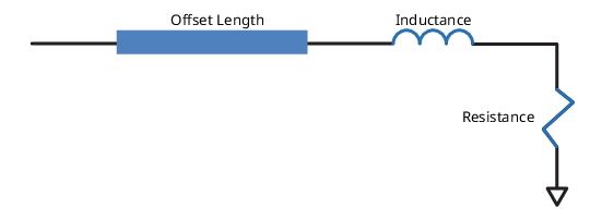
Load: Defined by a resistance, an inductance and an offset length relative to the desired reference plane. The resistance and inductance are in series as shown in the diagram below.
Flex Standards Load Model
.s1p-Defined: Defined by an S-parameter file for the standard supplied by the user. The values will be interpolated to match the current frequency list. If the file frequency list and the current list are incompatible (too small an amount of overlap), an error will be generated.
Considerable flexibility is given to the user on selecting the standards to employ but not all combinations will work. On 2 and 3 standards cases, the selections must produce different reflection coefficients at every frequency in the sweep range or singularities will occur. Checking is only done by the system to see if two identical standards are entered but even different entries can produce the same reflection coefficient. An example is a 2 standard, short open case where the short and open have different offset lengths. If, for example, the short offset length is 1mm and the open offset length is 2mm, the two standards produce the same reflection coefficient at 75 GHz. For lower frequency sweeps, this combination will work. The multiple offset short (or open) case also follows these rules as is evident from earlier chapters in this guide on SSST and SSLT calibrations.
The use of the load standard raises somewhat more complicated issues and is often only used in the 3-standards case. In the one standard case, it will raise uncertainties in the fixture insertion loss estimate if the load reflection coefficient is even close to as small as the mismatch of the fixture. In the two-standard case, similar issues happen except both the fixture match and insertion loss extractions can be imperiled. If the fixture is well-matched, the use of a load standard can improve the extraction of that mismatch.
.s1p files cover the gamut of the above possibilities but concept of independence still holds. The reflection coefficients of the various standards (in a complex sense) should be as far apart as possible for maximum accuracy.
The 'Classical open-short' selection is a special case of the 2-standards scenario where a zero offset open and short are used and the fixture arm is assumed to be electrically short. This assumption, most often used in on-wafer de-embedding scenarios, enables more detailed match information about the fixture/lead-in to be determined at the expense of generality.
In the space of this chapter, it would be difficult to cover the sensitivities for all possible combinations of fixture parameters and standards. We can, however, offer some examples that might illustrate some of the trends.
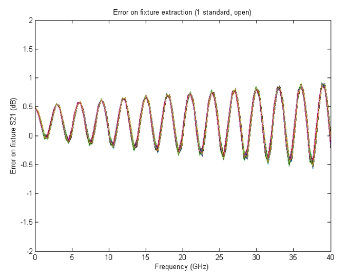
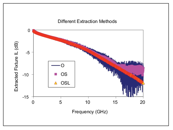
Consider the one standard case first where the fixture has 25 dB return loss (flat with frequency) and has 5 dB of insertion loss at 40 GHz (going to 0 dB at DC with a square-root-of-f dependence). In the first experiment, an open will be used and a Monte Carlo simulation run where the reflection coefficient magnitude (which should be 1) is allowed to vary +/-5% and the phase is allowed to vary +/- 10 degrees. The errors on extraction look like that below. The width of the apparent trace gives the sensitivity to the standard changes which is quite slight. The macroscopic curve is the error for ignoring the fixture match (by using 1 standard only). Clearly the standard sensitivity is not a huge problem. Since the loss of the fixture gets closer to the mismatch at higher frequencies, the error increases.
Error On Fixture Extraction (1 Standard, Open)
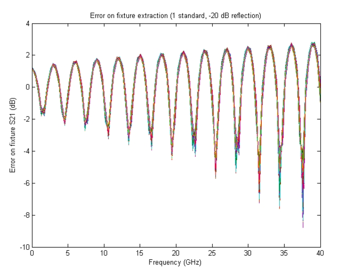
Now consider the case where the standard is a 20 dB return loss device and we run the same simulation. The standards sensitivity has increased in this case (width of the composite trace) although the scaling of the magnitude variations used may not have been comparable. The overall errors increased since the measured insertion loss contribution to the reflection measurement is now even smaller relative to the (ignored) fixture mismatch.
Error On Fixture Extraction (1 Standard, –20dB Reflection)
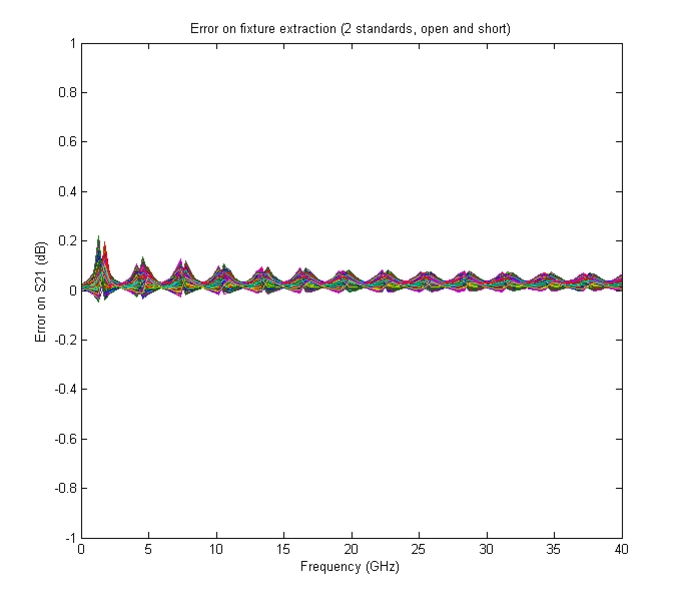
Moving to the two standard case with roughly the same fixture (except now |S11|= –25 dB and |S22|= –20 dB). First, an open and a short were used with the same 5%, 10 degree parameter variation. The resulting errors are now much smaller since some mismatch is being accounted for. The standards sensitivity is now a much larger fraction of the error. The errors are also now larger at lower frequencies since the lower loss exposes the mismatch asymmetry of the fixture more to the measurement.
Error On Fixture Extraction (2 Standards, Open and Short)
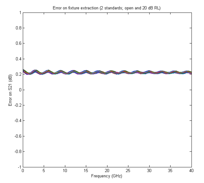
If the 20 dB return loss device is substituted for the short, the profile changes dramatically. Since one of the standards is similar to the fixture match, the deconvolution of loss and mismatch extraction in this method breaks down somewhat so the error increases (although it is still much better than with one standard).
Error On Fixture Extraction (2 Standards, Open and 20 dB RL)
In the three-standard case, there are an even larger number of variations but, since the input and output match are being solved for independently, the sensitivity and errors will decrease as long as the standards level-of-knowledge remains constant. One example comparing one, two and three standards is shown below. The mismatch of this fixture is relative symmetric and below –20 dB until about 10 GHz and degrades to about –10 dB by 20 GHz (and becomes less symmetric). One can see the one-standard approach starting to diverge relatively early as the fixture mismatch becomes increasingly significant relative to the insertion loss. The two-standard approach starts deviating later only when the match asymmetry becomes more significant.
Extracted Fixture Example Comparing One, Two, and Three Standards
As a summary of all of the Type B permutations:
• A full standards version (or flex standards with 3 independent standards) can produce the best possible accuracy and lowest sensitivity but only if the standards are well-known. To put it another way, the ‘performance ceiling’ is the highest.
• Flex standards with two independent standards can do very well if the fixture arm is relatively symmetric and does particularly well when the insertion loss is low. An open-short pairing is the most common and is a favorite in on-wafer and micro-fixture applications. This approach fares less well with higher loss, asymmetric fixture arms.
• Flex standards with one standard is sometimes the only practical method due to the interface on the far end of the fixture. A high reflection is the best choice for that standard usually unless the fixture is exceptionally well-matched. This approach is most accurate when the fixture mismatch is very low.
Quick Extract
The Quick Extract check box disables the file entry fields and instead saves the output file to a pre-determined location and automatically starts the de-embedding engine. The file just saved will automatically be loaded into the de-embedder (where it can be edited). This process can help save time if the desire is to immediately de-embed a fixture that was just extracted. Note that any de-embedding in place prior to the extraction will be cleared (and the system will warn if this is about to happen). If de-embedding was on when extraction was run, those de-embedded values will be used during extraction so some caution is advised as it is possible to partially negate an extraction by using already partially-de-embedded data.
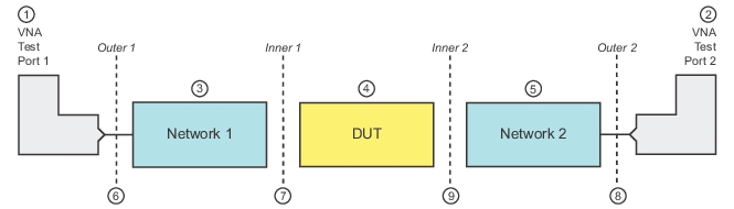
Type C Network Extraction
Type C is the most complete, dual fixture extraction approach offered in the VNA. It requires full 2-Port calibrations at two sets of reference planes but can fully determine the S-parameters of two networks independently.
Consider the diagram in NETWORK EXTRACTION dialog box (above in Figure: NETWORK EXTRACTION Dialog Box—2-Port VNAs (Option 21 Enabled)). A calibration is required at the outer reference plane set and the inner reference plane set. The outer calibration can usually be done coaxially (or some other well-defined media) depending on the networks involved. The inner calibration is often more complicated and may be board- or wafer-level (and may require the user create calibration standards). Assuming these calibrations are possible, then the S-parameters of Network 1 and Network 2 can be found.
Network Extraction Process Diagram for Type C Networks
1. Test Port 1
2. Test Port 2
3. Network 1 attached to Test Port 1
4. DUT attached to Network 1 (on left) and Network 2 (on right)
5. Network 2 attached to Test Port 2
6. Outer Reference Plane 1
7. Inner Reference Plane 1
8. Outer Reference Plane 2
9. Inner Reference Plane 2
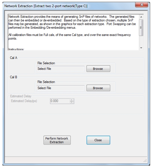
Two port calibrations at two different reference plane sets are used to extract the S-parameters of the intervening networks (often test fixtures). The dialog for loading the two calibrations is shown in NETWORK EXTRACTION [Extract Two 2-Port Networks (Type C)] dialog box below in Figure: NETWORK EXTRACTION Dialog Box—Extract Two 2-Port Networks—Type C.
NETWORK EXTRACTION Dialog Box—Extract Two 2-Port Networks—Type C
As before, the two calibrations are performed and the setups saved, typically as an active channel CHX file type.
Some conditions:
• The two calibrations must be full 2-Port cals and must have the same frequency lists.
• After extraction is performed, a file dialog will appear allowing the user to indicate where the S2P files should be stored.
• The networks are assumed to be reciprocal.
Unlike Types A and B, this method determines the two fixture halves completely and independently. As a trade-off, a complete set of standards at the inner plane are now required. Algorithmically, this type is very similar to Type A except two networks are processed simultaneously. If the inner cal standards can be successfully made/acquired, the inner match values extracted will typically be more stable than those acquired with a Type B analysis for the reasons discussed in the previous section.
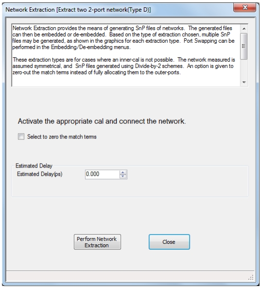
Type D Network Extraction
The dialog is a very simple one and is shown in Figure: NETWORK EXTRACTION Dialog Box—Extract Two 2-Port Networks—Type D (without Option 21). The outer calibration should be active when this procedure is called since files are not recalled as with the other techniques. Because it is sometimes difficult to allocate or interpret the match terms, a check box is provided to ignore those terms altogether. In this case, S11 = S22 = 0 (linear) in the exported S2P file. As with the other techniques, a dialog will appear upon execution to allowing the naming of the destination S2P file.
NETWORK EXTRACTION Dialog Box—Extract Two 2-Port Networks—Type D (without Option 21)
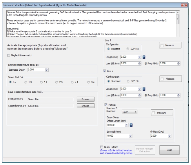
Type D Network Extraction—Multi Standards (with Option 21)
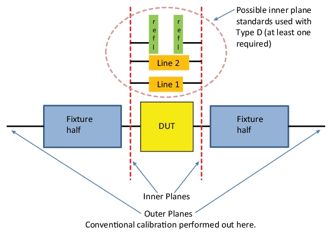
Type D is considerably different from the other techniques (except some configurations of flexible standards in Type B) in that it relies only on a limited number (1-3) of measurements to extract parameters rather than relying on the manipulation of a pair of calibrations. A full 2-port calibration is performed at the outer planes (often in coax or waveguide or with on-wafer probes) and then simple standards (one or more lines and possibly a single high-reflect standard) are connected between the fixture halves as suggested in Figure: Network Extraction Type D. The non-Option-21 version of Type D differs in that only a single line standard is allowed and its length must be 0.
This technique belongs to a class of approaches that have been termed ‘partial information techniques’ since they make additional assumptions about the fixture to avoid the necessity of a full calibration at the inner plane. As such, these techniques are particularly attractive when the inner plane has a complex structure or geometry that makes it difficult to create many standards for that plane or difficult to accurately model those standards. There are also cases where such methods are useful because the repeatability of connection at the inner plane is degraded. By de-emphasizing inner plane match in those cases, sensitivity to repeatability issues can be reduced.
There are a number of different ways to use Type D and this section will explore the differences and how one might choose the sub-approach to take. In earlier versions of the VectorStar software (prior to 2017), only one choice was available: the use of a zero-length thru between back-to-back fixture halves which assumed that the halves were identical and had perfect match at the inner plane. That sub-approach is still available, as will be seen, but there is now more flexibility.
Network Extraction Type D
The basic structure of Type D extraction is shown here. There is considerable choice in the standards used at the inner plane, but the combinations all share the fact that the set is not ‘complete’ in the sense of a full calibration at that plane. Some fixed error is accepted in exchange for simpler standards and more immunity to repeatability issues.
NETWORK EXTRACTION Dialog Box Type D Multi-Standards (With Option 21)
The basic Type D extraction starts with a line between fixture halves as mentioned and will assume symmetry of the fixture halves. This line can have any length but that length must be specified and any errors in that specification will map through to the phase lengths of the extracted fixtures. If one stops here, the mismatch at the inner planes of the fixture will be ignored (S22 will be zero in the extracted files). One can also elect to set all match terms to zero and that will force both S11 and S22 to zero no matter how many standards are used. This zero-match choice can be useful if repeatability at the inner plane is particularly poor and insertion loss/phase correction for the fixture is the primary concern (doing a closer-to-full match correction with a very non-repeatable interface can often further reduce the transmission extraction accuracy). A fixture length entry is requested (represents both halves together) and this is used just for root selection so precision is not normally required. If zero is entered for the fixture length, an automatic routine (similar to auto reference plane extension discussed in Calibration and Measurement Enhancements of this guide) is used to estimate the length.
One can also add a second line of some different length (and its transmission amplitude can be entered independently) and inner plane match will no longer be ignored. Note, however, that the accuracy of the entered line lengths is more important in this case. Also, the line length difference between the first and second lines should not approach 180 degrees within the frequency range of interest (or be too close to 0). Generally, the line length difference should be between ~10 and 160 degrees over the frequency range of concern.
The use of reflection standards (which must be placed on the inner planes of both fixture halves) will also allow for solving for inner plane match. Finally, one can use all three standards which will generally improve accuracy on both insertion loss and inner plane match. The choice on how many of the standards to use should depend on how well those standards can be made (e.g., can a second line length be made that is still relatively well-matched as a transmission line, can reflect standards be made that have relatively uniform reflection magnitude over the frequency range of interest, etc.). Implicit in this is that the measured characteristics going from the first standard to the second standard do not change for other reasons (e.g., if the structures being measured are different implementations of the same fixture, then they must be quite identical). Note that while fixture symmetry is implicit for all of type D, the sensitivity to asymmetries is heightened with the use of the reflect standard. Generally, if additional standards perform well in this sense, using them will improve the overall extraction.
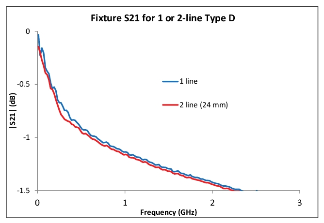
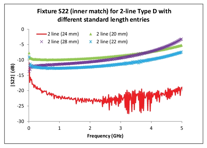
As an example, consider the measurement of a back-to-back cable assembly where two different thru lengths are possible at the inner plane (0 and 24 mm). If one compares the single line approach to the two line approach on extracted insertion loss, one can see some differences (Figure: Comparison of Single and Double Line Type D Extractions of Insertion Loss). The single line approach produces an insertion loss with slightly more ripple and a slightly more optimistic overall value (although errors in either direction are possible).
Comparison of Single and Double Line Type D Extractions of Insertion Loss
A comparison of single and double line Type D extractions of insertion loss are shown here. With a correct standard length entry and sufficient repeatability, the double-line method can increase accuracy of the extraction.
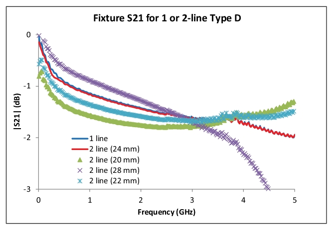
If the entry of the standard line length is not accurate, however, substantial errors can result. The extraction of the previous figure is repeated in Figure: Resulting Error with Inaccurate Standard Line Length Entry for the added cases when the 2nd line length is off by ~10 or 20 %. The errors are a few tenths of a dB at low frequency but grow larger at high frequencies as the standing wave that is being corrected grows more dense. Also, in this case, the 28 mm entry brings a singularity to lower frequencies and this has an even more substantial effect on the error.
Resulting Error with Inaccurate Standard Line Length Entry
One reason for using the two line approach (or line+reflect) is to get more reasonable values for inner plane match which can be important for sequential de-embedding and modeling. Again, the parameter entry accuracy is important for the inner plane match as it was for insertion loss extraction. The inner plane match values for the fixture of Figure: Resulting Error with Inaccurate Standard Line Length Entry are shown in Figure: Inner Plane Match Values for the same length entries.
The single-line version of Type D is best obviously for well-matched fixtures relative to loss (i.e., very well matched if low loss and moderately well-matched for moderate loss). With a 20 dB return loss, there will be generally 0.3 dB or more of insertion loss uncertainty with this technique (as opposed to ~<0.1 dB with other techniques if good standards are available). With a 10 dB return loss fixture, it will be several dB of uncertainty. With additional standards (assuming accuracy of length entries and sufficient repeatability), the method becomes more mismatch tolerant—often keeping errors under 1 dB for a 10 dB return loss fixture—but the results will still be worse in an absolute sense than with a complete method (assuming the latter was possible).
Additional Notes Regarding Type D—Multi-standards
• A full 2-port calibration must be active and the extraction will be run over that frequency range. For 4-port systems, at least a full 2-port calibration must be active (more details on the 4-port cases are covered in Multiport Measurements of this measurement guide).
• The line and reflect offset lengths are entered in millimeters, although a calculator is available if values are in picoseconds. If the material type is set up (from the current calibration or manually thereafter), that and any active dispersion relations will be used in the calculations. In two-line cases, the first and second lines must be electrically distinct (i.e., phase length differences not too close to 0 or 180 degrees within the frequency range of interest).
• -The Quick Extract feature (allowed on all type D variations with option 21) suppresses the file name entry fields and instead saves the files to a predetermined location, automatically opens the de-embedding engine, and loads the just-generated files into the de-embedder. These entries can be changed at that time if desired, but this process can save time if the desire is to immediately de-embed a fixture that was just extracted.
• The Measure buttons are used to measure the two fixture halves with the appropriate standard connected and those standards must be connected when the relevant Measure button is pressed. The system will trigger a channel sweep at that time to acquire new data.
• Loss of the line and reflect standards can be entered that scales with length and frequency (in a sqrt(f) sense relative to the entered reference frequency; if a zero reference frequency is entered, the loss will be assumed constant with frequency).
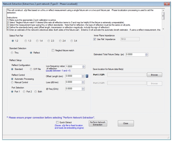
Type D Network Extraction—Phase Localized (with Option 21)
Another variation of Type D is termed ‘Phase Localized’ where a single standard (either a line or a reflect/reflect pair) is used along with the assumption that the fixture is electrically long enough (based on the frequency range being used) and the bulk of the fixture mismatch is not too close to the inner plane. The dialog for setting up phase localized extraction is shown in Figure: NETWORK EXTRACTION Dialog—Type D—Phase Localized (With Option 21).
If the assumptions are met, this method can outperform the previously discussed Type D variations. More central to this method is the fixture length as transmission-line-like: functions are cross-correlated with the measured data to better isolate insertion loss and reflection coefficients of the fixture halves. If the fixture length entry is set to zero, an automatic process (much like auto reference plane delay discussed in Calibration and Measurement Enhancements of this guide) will estimate the length. As before, entries for the line length or reflect offset length are required and any errors in those values will translate to extracted parameter phase. If the line is chosen as the standard, symmetry between the fixture halves in terms of insertion loss will be assumed. If the reflect standard is chosen, no symmetry is assumed and only one half of the fixture can be extracted if desired. If both halves are to be extracted, length estimates for the individual arms can be entered. In this variation of Type D, there is no Measure button and the measurement is executed when Perform Network Extraction is selected.
Finite transmission of the thru standard (or .s2p definition) can be entered as can loss of the reflect standard. As with some other network extraction methods, the reflect loss is entered in dB/mm terms and the value will scale with frequency (as sqrt(f/fref); if fref=0, the loss will be treated as constant with frequency).
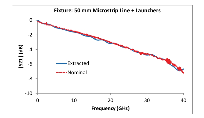
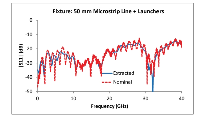
As an example, consider a fixture consisting of a ~50 mm microstrip line, a coaxial launcher on one end and a DUT-local launcher on the other end (for each arm of the composite fixture). Suppose only an open standard is available and one would like to use the phase-localized approach since there was only the one standard and it was believed that most of the mismatch was away from the DUT interface. In this case, it was possible to do a complete calibration at the inner reference plane so a comparison was possible. The extracted vs. nominal insertion loss is shown in Figure: Microstrip Line Example (1 of 2). One can see pretty good agreement until about 30 GHz when it did work out that DUT-plane mismatch on the fixture was getting large. Further, the fixture started having significant radiation above about 35 GHz which further complicated the extraction. The return loss (extracted and nominal again) values are also plotted in Figure: Microstrip Line Example (1 of 2) and again show reasonable agreement until the very high frequencies. Recall that uncertainty in return loss in dB terms gets much larger as the match gets very good just based on a residual directivity argument (a few dB at the -20 dB level for a decent coaxial calibration).
This example does reinforce a couple of points:
• Partial information methods do have some fixed error because of the incomplete ‘calibration’ at the inner plane
• The further the fixture deviates from the ideal aspects assumed by the method (where mismatch is located in this case), the larger those errors become.
Still, if it was indeed only possible to have an open standard for this fixture, the results shown here are better than one could achieve with a single-standard generalized B method or with a simple normalization.
Microstrip Line Example (1 of 2)
The results for a phase-localized Type D extraction are shown here along with nominal results for a special case when both port of the fixture arm were connectorized (to allow for comparison). The extraction degrades at higher frequency as fixture radiation and inner-plane mismatch hamper the partial information technique. Only an open reflection was used for the extraction process.
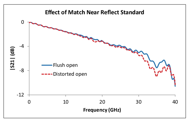
The direct sensitivity to standards definition defects are fairly straightforward since the reflection or transmission coefficient entered is applied multiplicatively to the data prior to a square-root operation. More subtle are non-idealities in the standards (such as mismatch of the line/thru standard). This will have impact through its influence on actual insertion loss during the measurement (in terms of an offset loss and in terms of ripple). Also on the subtle side are the effects of an incorrect fixture length entry. While in normal Type D this is mainly used for root choice, it is used in phase-localized D to determine which phase signatures to correlate against so entering a significantly incorrect value (10s of mm generally) can cause added ripple and, eventually, drop outs in insertion loss extractions as well as incorrect return loss values. The internal length estimate approach (entering 0 in the fixture length estimate field triggers this) can reduce the issues and is recommended unless the fixture phase response is very resonant, in which case a proper manual estimate will yield better results. The issue of where the mismatch is predominantly located was touched on earlier. This has somewhat more of an effect when using the reflect standard (since the fixture mismatch and the reflect standard are almost co-located so phase localization becomes difficult) than using the thru/line standard. As an example, consider the extraction of a microstrip section using a flush open reflect standard native and when the mismatch near that standard has been distorted from the original ~ –15 dB to ~–5 dB at high frequencies. The effects on fixture |S21| are shown in Figure: Inner Plane Match Values: added ripple and some substantial differences above 30 GHz (where the mismatch change was the largest).
Inner Plane Match Values
To further explore the sensitivity to inner-plane mismatch, a (reflect-based) phase-localized D extraction was performed on an original fixture and again after additional mismatch was introduced. In the range of additional mismatch addition, the discrepancies increased as expected.
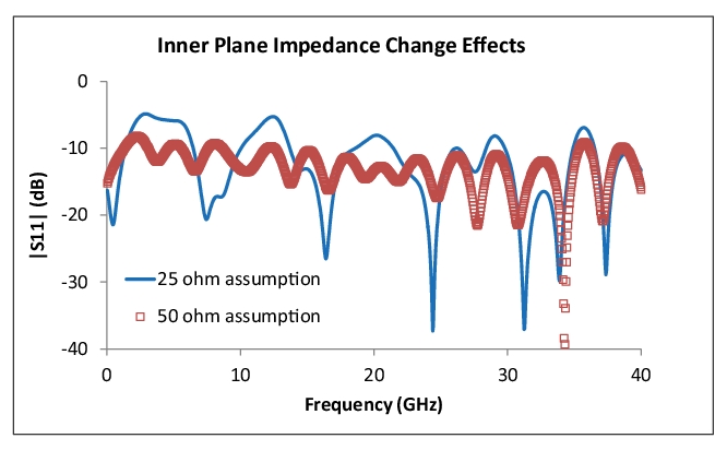
Fixtures with distinct impedance changes, intentionally constructed or otherwise, present an additional challenge. Consider a fixture where the inner plane is at 25 ohms and a thru standard is used for the extraction. If the inner plane impedance is ignored, then one is essentially treating the half fixture as being terminated in a 25 ohm impedance (low reflection for that zone) but that is implicitly changing the reference impedance of the S-parameter matrix. While this may sometimes be desired, it will cause errors if not anticipated when using that file for later de-embedding of modeling. More conventional is to keep the reference impedance (of the matrix) consistent at 50 ohms to facilitate later processing. In this case, the difference in the match parameters is substantial as shown in Figure: Phase Localized Type D Extraction—Effects of Inner Plane Impedance Change.
Phase Localized Type D Extraction—Effects of Inner Plane Impedance Change
In a (thru-based) phase-localized D extraction, inner plane impedance deviations can create issues if large enough. In this case, the inner plane was at 25 ohms while the launch (and reference impedance for the calibration) was 50 ohms. If the impedance change was ignored (red squares in the plot), the extracted return loss for the fixture half can be significantly in error.
Additional Notes:
• A full 2-port calibration must be active and the extraction will be run over the current frequency range (which is a subset usually of the calibration frequency range). For 4-port systems, at least a full 2-port calibration must be active (more details on the 4-port cases are covered in Multiport Measurements of this measurement guide). There is a requirement that the frequency list have nearly uniform frequency steps (an individual step size cannot deviate from the mean by more than 5%) so some segmented sweep setups (and all log sweep and CW setups) will not be accepted.
• The frequency range of the sweep should be large enough that the total fixture length (ns)>5/(frequency range (GHz)). The frequency step should be small enough that the total fixture length (ns) < 0.3/(Frequency step (GHz)). This helps avoid insufficient phase slope or phase-wrap-aliasing (respectively) that would complicate phase localization.
• The line and reflect offset lengths are entered in millimeters although a calculator is available if values are in picoseconds. If the material type is setup (from the current calibration or manually thereafter), that and any active dispersion relations will be used in the calculations.
• The extracted results are stored as .s2p files with port 1 of each file being the outer plane. Details of the file format options (frequency units, etc.) are set by the entries on the sNp setup dialog. See Table: Standards Requirements for Generalized B and Type D Extractions for recommendations of extraction types and standards needed for various fixture behaviors.
Standards Requirements for Generalized B and Type D Extractions
Method
Standards Needed
Best for Fixtures
Generalized B
Open
Open/Short
Well-matched fixtures with very well-matched inner plane. Reflection-only standards possible
Existing D
Thru
Well-matched fixtures with very well-matched inner plane. Thru-line standard possible
Multi-standard D
2 lines
Line + (Open OR Short)
Moderately-matched fixtures without structural assumptions other than symmetry. At least one line standard possible. Good for high loss fixtures.
Phased-localized D
Line Or (Open OR Short)
Moderately mismatched fixture assuming most mismatch not at inner plane. No symmetry necessary. One standard only
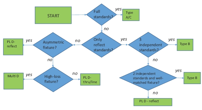
Another way of looking at method choice is with the flow chart shown in the Figure: .
Sequential Extraction—Peeling (with Option 21)
Another method of network extraction involves modeling the network as a collection of lumped elements. This is particularly popular for electrically small structures (e.g., on-wafer) of those with runs of transmission line punctuated by electrically small structures (e.g., PC boards with isolated vias in transmission lines). Procedurally, this method works on one lumped element at a time. For each element, a .s2p file is generated that can be de-embedded to allow one to get at the next element. Also transmission line segments can be separately de-embedded to get between lumped defect areas. The process is based on reflection measurements only and a full calibration incorporating that port must be in force.
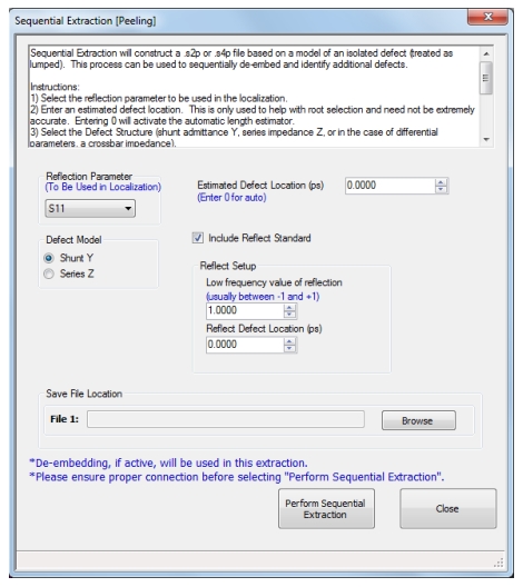
The basic method accepts as input the location (in time from the reference plane) of the defect area of interest and the type of element to model the structure: shunt admittance (Y) or series impedance (Z). A 0 can also be entered as the position and, in that case, an automatic calculation will be performed to select the largest remaining defect. A differential pair can also be selected in which case the model element is a crossbar impedance (between the two ports) and a .s4p file will be generated. The dialog is shown in Figure: Sequential Extraction Dialog.
Sequential Extraction Dialog
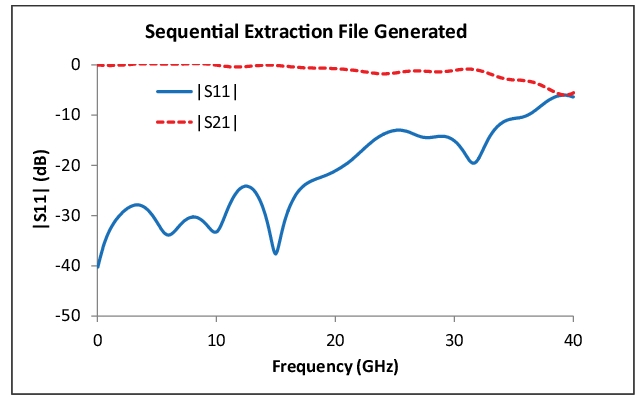
As an example, consider a fixture with multiple transitions but one is known to be particularly inductive (in a series sense). It might be interesting to look at the return loss of this fixture if that particular transition could be improved. It is known that this launch is about 120 ps in from the reference plane so the sequential extraction tool was used with that defect position entry and a Z-series element selection. A 2-port calibration had already been performed. The extracted .s2p file for the element shows the result in Figure: Sequential Extraction Plot. As might be expected, the return loss of the model element is indeed degrading with frequency and the insertion loss increases.
Sequential Extraction Plot
Values from the series network extracted for the example fixture are plotted here.
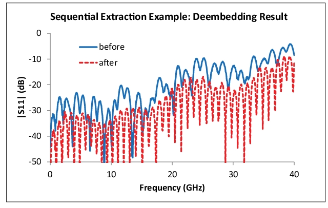
To remove this from the fixture result, two steps are needed: de-embed the 120 ps (air equivalent 36 mm) of transmission line and de-embed the file just generated. This was done and the before and after de-embedding results are shown in Figure: Sequential Extraction Example—Deembedding Result Comparison. Indeed, the inductive transition was responsible for a fairly large share of the overall fixture mismatch and improving that one transition could have significant benefits. The final result is not perfect since there are additional transitions in the fixture but also because this extraction is somewhat model-like: it is only valid if the defect is indeed series in nature (or shunt if the admittance version had been selected). In this particular case, the series model was a very reasonable choice.
Sequential Extraction Example—Deembedding Result Comparison
The before and after de-embedding return loss values of the example fixture are shown here.
The basic method is adequate for electrically small structures but inaccuracies can enter the picture if there are un-de-embedded losses between the reference plane and the defect center. An extension to this method can help compensate for these losses by using analysis of another, known reflection center. If there is a known reflection at the end of the fixture (e.g., an open or a short), the analysis of that response can be used to compute a loss estimate and correct the extraction of a lumped element representing a defect between the reference plane and the reflection standard. The reflection coefficient of the standard must be entered (must be real and normally between –1 and +1) and its position relative to the reference plane is usually entered. A zero (0) can be entered for the location and an automatic routine will be used to locate the largest response which is presumed to be due to the reflection standard. If an auto routine (0 entry) is also used for the defect location, the next larger response (distance less than that of the reflect standard) will be used for that item.
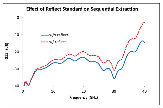
To see the effect of the reflect standard, consider the effort to extract the .s2p file for a via structure in a transmission line. The defect is located ~170 ps in from the reference plane but the transmission line is of fairly high loss. It is possible to place an open reflect standard at about 400 ps from the reference plane and that open is electromagnetically well-behaved at least to 40 GHz (our range of interest). The via structure will be modeled as a series impedance and the simple sequential extraction produces a file with the return loss shown as the solid curve in Figure: Sequential Extraction—Effect of Reflect Standard. If one also uses the reflect standard (position 400 ps, reflection coefficient = +1), one gets the dashed line instead. Ignoring the line loss up until the defect would have cause one to underestimate the defect return loss by nearly 10 dB at 40 GHz.
Sequential Extraction—Effect of Reflect Standard
As shown with this example, using the reflect standard to compensate for line loss can be useful if the defect is far from the reference plane in a lossy medium.