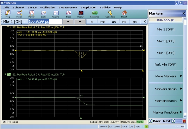
Low pass mode assumes the existence of data near DC which enables the ability to compute step responses and to create a pure real transform. While any graph type can be used (except Imaginary which would have a flat line), Real is sometimes the most valuable since information about the defect can be determined. An example plot showing a short at the end of a small transmission line length of approximately 100 ps appears in Figure: Example Low-pass Time Domain Plot. Both the impulse response and step response are plotted on real graph types. Many aspects of this plot will be discussed in this section including the impulse and step presentation of the same data.
Example Low-pass Time Domain Plot
Many of the other submenus change slightly depending on which mode is selected so the remaining subsections will be partitioned according to the mode.
The fundamental output of the transform depends on the non-dispersive or dispersive nature of the media. In the case of non-dispersive media (to include coax), time is the fundamental output of the transform and distance is calculated using the media information on the measurement menu. In the case of dispersive media (waveguide or microstrip), distance is the fundamental output and time is calculated from that.
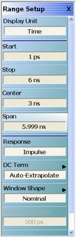
The Start, Stop, and Center buttons all invoke field tool bars that allow user-input for each value (in distance or time); with the Span button displaying the calculated result. There are few limits to what may be entered but extreme entries may not always be useful due to constraints of resolution and alias-free range. These limits are determined by the frequency list used as well as the window selected.
Resolution is interpreted as impulse width (the width of a singular defect) while alias-free range is the maximum time range that can be studied before defects start repeating themselves (due to the cyclical nature of the transform). To help, the resolution (impulse width) is displayed as a read-only variable on the main time domain menu (Figure: Domain Menu Variations Based on Time Domain Mode Selection (1 of 2)) and the alias-free range is displayed on this range menu as a read-only variable.
The response choice is either Impulse or Step. The step response, which allows a TDR-like display is simply an integration of the impulse response which is the natural output of the transform. Normally, this integration begins at the start time used in the current range (and continues to the stop time). This is advantageous when using results for certain de-embedding activities. It can, however, be confusing if one zooms into a region of impedance different from the reference impedance since the integration would not capture the transition. For this reason, there is the selection available to start the integration at 0 (regardless the range setting). The integrated result will be mapped back into the current start-stop range using interpolation with the linear value set to zero at negative times. If the stop time is also negative, the integrated result will all be near zero.
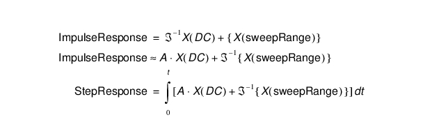
Note that the integration for step response also requires an initial integration value and this comes from the network’s DC response. Since the VectorStar MS464xB VNA cannot get all the way to DC, some additional information is needed to perform this integration. To see this consider:
Equation 14‑1.
DC Term Menu
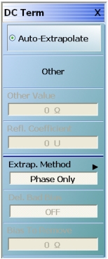
Since the DC value ends up being integrated from time 0 (zero), the value used here is quite important and the choices to compute this value are shown in Figure: DC TERM Selection Menu. The default choice is to allow the system to auto-extrapolate from existing frequency data to estimate the DC value.
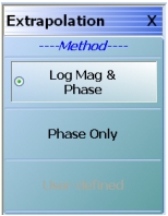
The default method, Mag-Phase, extrapolates both portions as would be expected and is energy-conserving. For cases where the start frequency is low and the DUT loss changes slowly over frequency, sometimes the magnitude may be assumed constant and only the phase function need be extrapolated (most common with long cable assemblies). The other option allows a table of low frequency values to be entered (two-column, tab-delimited). If the DUT is well-known, extrapolation can be avoided altogether by entering the DC impedance.
Window Shape Menu
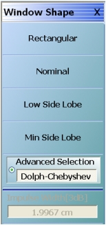
The last item on the Range Setup menu is the Window Shape selection button which displays the Window Shape submenu shown in Figure: WINDOW SHAPE Menu.
WINDOW SHAPE Menu
Since the frequency range of the VNA is finite, the frequency domain data will have a discontinuity at the stop frequency. This introduces side lobes in the time domain data that can obscure smaller defects and hamper separation of defects. The window provides some pre-processing of the frequency domain data to reduce the severity of the discontinuity and hence the side lobe level. This also reduces resolution but is unavoidable.
The Nominal window is the default and provides about half of the resolution of Rectangular (no window) but with an approximate 30 dB reduction in side lobe levels. The Nominal window is advised for most applications.
Since the window so strongly affects resolution, the Impulse Width display is repeated on this submenu to help determine the impact on the desired measurement.
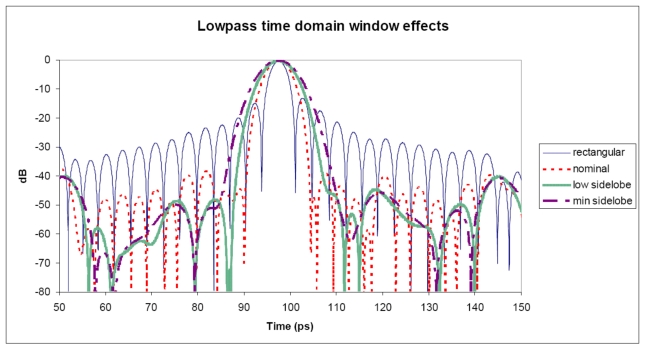
An example of how the window shapes affect the impulse data (main lobe width and side lobe level being traded-off) is shown in Figure: Effects of Window Shapes Plot. Here the same data appears with the four different window selections. For this plot, data was saved to TXT files and plotted externally.
Effects of Window Shapes Plot
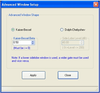
The Advanced Window selection button brings up the dialog shown in Figure: Advanced Window Setup Dialog that has the previous four choices along with two new parameterized windows, Kaiser-Bessel and Dolph-Chebyshev.
Advanced Window Setup Dialog
The dialog for advanced window setup makes two new window choices available (Kaiser-Bessel and Dolph-Chebyshev). The Apply button must be used for a radio-button selection to take effect.
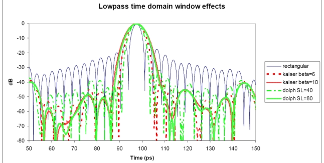
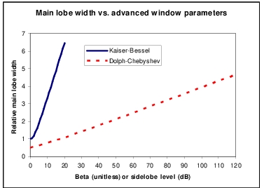
These two new window types allow for a finer selection of the trade-off between side lobe level and resolution. For the Kaiser-Bessel window, a larger Beta value leads to lower side lobes, but a wider main lobe width (and hence poorer resolution). For the Dolph-Chebyshev window, the side lobe level is parameterized explicitly (in absolute dB) and a larger value leads to a wider main lobe width as well. The windows for two parameter values for each of these windows are shown in Figure: Effects of Window Shapes Plot with Advanced Windows Selection along with the rectangular window for comparison.
Effects of Window Shapes Plot with Advanced Windows Selection
The approximate relationship between these parameters and the main lobe width (null-to-null) is suggested in Figure: Comparison of Lobe Width vs. Window Parameters. Here, everything is scaled relative to a rectangular window (a nominal window is at 2, a low side-lobe window is at 3, and a minimum side-lobe window is at 4 on this scale) and the y-axis is normalized relative to the lobe width of a rectangular window.
Comparison of Lobe Width vs. Window Parameters
o
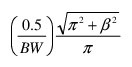
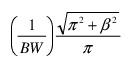
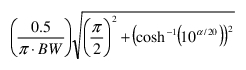
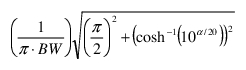
Below are the window widths (expressed in terms of the distance between the first nulls around the central lobe). ‘BW’ refers to the total sweep bandwidth.
Window Type
LP Main Lobe Width (null-null)
BP Main Lobe Width (null-null)
Rectangular
0.5/BW
1/BW
Nominal
1/BW
2/BW
Low sidelobe
1.5/BW
3/BW
Minimum sidelobe
2/BW
4/BW
Kaiser (parameter ß)
Chebyshev (parameter α dB)
Below are the window widths (expressed in terms of the width between the 3 dB points relative to the central lobe). ‘BW’ refers to the total sweep bandwidth.
 o
o