Uncertainties in Time Domain Measurements and Recommended Practices
Because native time domain results are an integral of the underlying frequency domain data, understanding the uncertainty in the results is not always intuitive. Consider a measurement of a single point reflect (with little frequency response) so the frequency domain reflection coefficient is:
Equation 14‑2.
Where K is the complex amplitude of the reflection (assumed frequency-independent for this example) and L is the distance from the reference plane.
In the time domain (impulse mode), this corresponds to a single impulse at length position L and a magnitude |K|. Now, in the frequency domain, there will be uncertainty including fixed and sloped offsets (from tracking errors, drift, repeatability…) and more complex distortions like ripple (from residual source match and directivity). As these are integrated over frequency, the fixed (in a dB sense) offsets pass‑through, sloped offsets have the potential to increase in effect, and ripple‑like errors have the potential to reduce in effect due to cancellation (depending on the frequency of the ripple). Immediately, this suggests that uncertainty components that may be of equal weight in the frequency domain may have a very unequal weighting in the time domain representation.
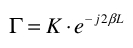
One can look at a simplistic case of a single, relatively large reflection and run Monte Carlo simulations of the effects of various uncertainty terms. Figure: Monte Carlo Scatter from a Simulation with Elevated Residual Source Match and Directivity Terms is an example where source match and directivity terms were elevated (to about the 20 dB residual level) and 1000 iterations were run with random component phases in the measurement. The net scatter was only about 0.1 dB which is noticeably less than the frequency domain uncertainty for a –12 dB reflection. This arises from the correlation between the corrected reflection coefficients at different frequencies.
Monte Carlo Scatter from a Simulation with Elevated Residual Source Match and Directivity Terms
The Monte Carlo scatter from a simulation with elevated residual source match and directivity terms is shown here. For a single spot defect, these error terms do not have a lot of effect on the time domain result.
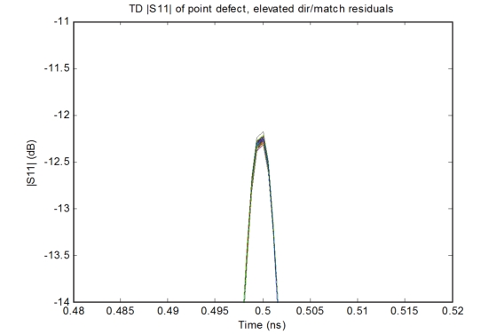
Monte Carlo Scatter from a Simulation with both Elevated Source Match/Directivity Residuals and an Elevated Drift Term
The Monte Carlo scatter from a simulation with both elevated source match/directivity residuals and an elevated drift term is shown here. The effect of the drift error in frequency domain has a major impact on the time domain result.
To understand this last concept, recall that the windowing de‑emphasizes the extreme frequencies of the data and an aggressive window removes quite a lot of that data. When the structure being tested is complex, the useful information tends to be spread over a wider bandwidth, hence it is more likely that windowing choice may have an impact on the result. In the first example (Figure: Results for Two Different Windowing Choices for Isolated Time Domain High-reflection Point), the DUT consisted of a single large reflect and two very different Kaiser-Bessel windows were used (ß=0.5 and ß=12). In terms of the peak amplitude, there is less than 0.03 dB difference.
Results for Two Different Windowing Choices for Isolated Time Domain High-reflection Point
The difference in results for two different windowing choices is shown here in the case of an isolated time domain high-reflection point. In terms of peak amplitude, the window choice [Kaiser-Bessel with parameter ß= 0.5 (red) or ß = 12 (blue)] had little effect.
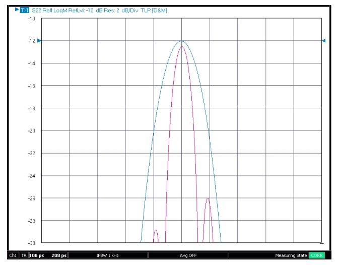
In the next example (Figure: Results for Two Different Windowing Choices with 2nd Time Domain Defect), the portion of interest is a –12 dB reflection and there is another ~ –25 dB reflection 70 ps away. In this case, the window choice makes a much larger difference with the aggressive window (ß= 12) being less correct. The salient difference here is the presence of a non‑negligible secondary reflection that is only a few resolution-widths away. This simple example illustrates that time domain uncertainty analysis is much more DUT‑dependent than is frequency domain uncertainty analysis and very different effects can dominate. For assistance in evaluating the uncertainties in particular situations, contact Anritsu.
Results for Two Different Windowing Choices with 2nd Time Domain Defect
This experiment is similar to that shown in Figure: Results for Two Different Windowing Choices for Isolated Time Domain High-reflection Point, except there is a 2nd time domain defect (about 13 dB lower in amplitude) positioned 70 ps away. In this more complex time domain structure, the window choice [Kaiser-Bessel with parameter ß= 0.5 (red) or ß= 12 (blue)] had a much more significant effect.
When one looks at step response time domain, there are additional issues in that the result is a time integration of the transform integration. In some sense, this secondary processing compounds the problems already discussed. One dominant aspect of this is the DC term discussed previously. Since the DC term transforms to a constant offset in the impulse response data, the step response will acquire a slope which can dwarf the actual reflection changes if the integration time is long enough. To add another layer, impedance is often plotted in step response and that represents another transformation. Combining these, one gets a reasonably complicated total transformation.
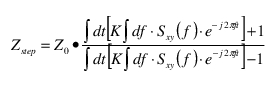
Equation 14‑3.
The main added uncertainty effect in the impedance transformation is one of sensitivity expansion at extreme impedances. Since the impedance changes more for a given S‑parameter change (usually reflection) as one gets further away from Z0, any of the earlier effects will be magnified for very high or very low impedances.
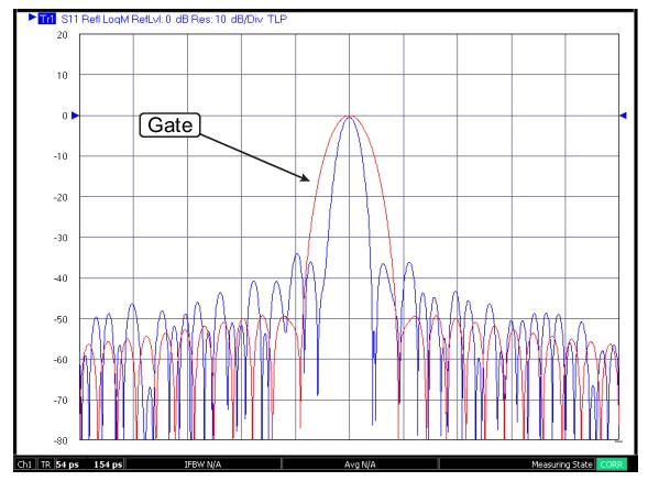
Shifting from time domain representations to the additional transform back to frequency domain (gating), one can also see a complicated uncertainty picture as alluded to earlier. Because of the windowing process, some information is lost in getting to the time domain which cannot be recovered. In addition, if the gate is on the order of resolution in width, then additional distortions occur due to the gate and window shape interactions. It is easy to envision the problem scenario in the plot below (Figure: Selection of a Gate that is Getting Narrow Relative to Resolution). The central lobe and its sidelobes represent the information about the defect to be analyzed. Since the gate is cutting off some of that information, the FGT response is now a distorted representation of that defect. While such an analysis may be useful in some cases, it is not a typical de-embedding‑like application where one is trying to remove secondary defects.
Selection of a Gate that is Getting Narrow Relative to Resolution
The selection of a gate that is getting narrow relative to resolution is shown here. This choice will tend to increase errors if frequency‑with‑time‑gate results at extreme frequencies.
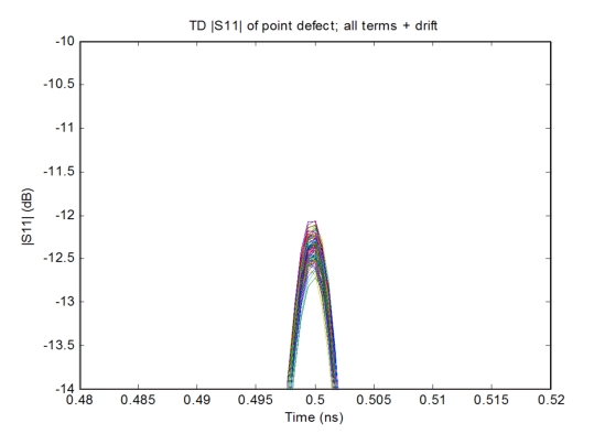
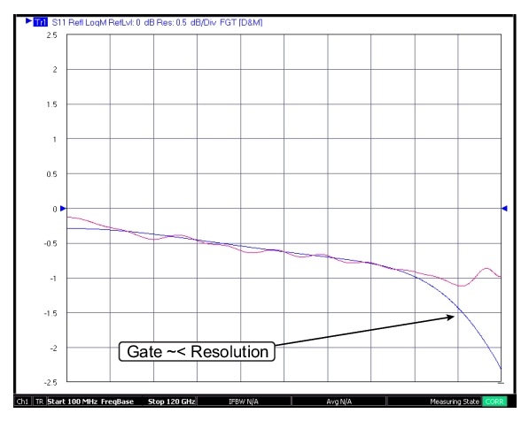
An example is shown below (Figure: Frequency-with-time-gate Result) where two different gate widths were used to isolate the same point defect in reflection. In this case, the wider gate was actually a bit too wide in that some secondary reflections remained resulting in the midband ripple. The narrow gate was, however, too narrow and resulted in major distortions at high and low frequencies. Note that this is a common occurrence: as the gate width gets too narrow the errors will increase first at the extreme frequencies.
Frequency-with-time-gate Result
A frequency-with-time-gate result for two gate width choices: one that is probably too wide for optimum isolation (red) and one that is probably too narrow (blue).
Optimizing Time Domain-related Uncertainties
Summarizing some of the above analyses, one can arrive at some general recommendations for optimizing time domain-related uncertainties:
• Do not use a more aggressive gate than necessary to get the sidelobe levels where needed. If there is a particular low-level defect near a large defect that needs to be identified, one of the parameterized advanced windows may be helpful.
• Pay particular attention to cable motion and drift if time domain uncertainty is critical.
• If using step response (or in some cases, frequency with time gate), pay attention to the lowest frequency used. A lower start frequency (if the DUT bandwidth permits it) can allow better DC extrapolation and more accurate step integrations. A lower IF bandwidth and/or averaging can also help in this regard.
• When using gating, do not select a gate shape that is more aggressive than needed and do not make the gate narrower than needed to isolate the defect of interest. The frequency extremes are most likely to be affected when the gate is inappropriate.