One feature in the time domain system is the ability to calculate an eye diagram representation of what the currently measured trace data would do to a digital data stream (that can be configured by the user). This is particularly valuable in seeing the data stream signal integrity issues that could occur with a given transmission path and can help with building up subsystem simulation results. Since the eye diagram computation is per-trace, one can configure a single channel having frequency domain, time domain impulse response, TDR-like and eye diagram traces simultaneously and all responding to the same live data.
Eye diagrams have been discussed extensively in the literature, but the basic concept is that they represent a data stream that has passed through an analog channel and it is fundamentally an analog data object where level and transition distortions can be analyzed. In this sense, it is a natural extension of VNA measurements.
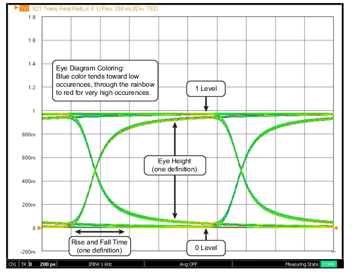
A generic eye diagram plot shown in Figure: Generic Eye Diagram Plot illustrates some of the key attributes that will be discussed.
A “heat map” type of plotting is used for eye diagram plotting with the color tending to blue for low occurrences and working up through the rainbow to red for very high occurrences.
Generic Eye Diagram Plot
There are a few general comments that can be made about the eye structure in Figure: Generic Eye Diagram Plot. The more the insertion loss increases with frequency, the softer the edges will become and the eye will further close in from the sides. Lower frequency defects may create structure throughout the eye, not just the edges. Jitter will cause a general edge broadening while additive white Gaussian noise (AWGN) will cause a more complete line broadening.
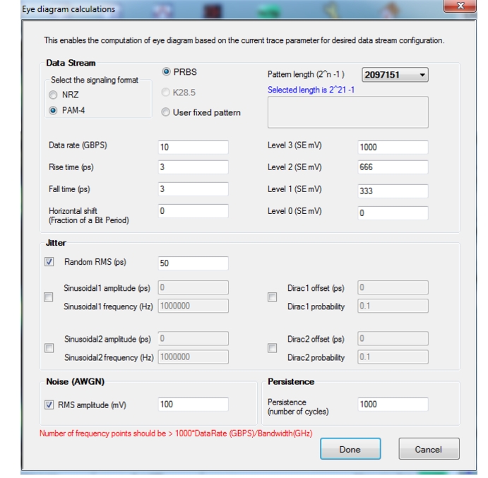
EYE DIAGRAM CONFIGURATION Dialog
The data stream parameters are configured on the eye diagram calculation setup dialog shown in Figure: EYE DIAGRAM CALCULATION Dialog. The signaling format is the first choice: NRZ (non-return-to-zero, the standard binary waveform) or PAM-4 (the four-logic-level discrete signaling format where each symbol contains 2 bits of information). The type of data stream is the next choice, with a Pseudo-Random Binary Sequence (PRBS) being the default. A user fixed pattern (up to 64 bits that then repeats) and the K28.5 standard (ISI maximizer, only available for NRZ signaling) are also possibilities. The data rate defines the symbol period that will be used for the evaluation. The high and low levels (1 level and 0 level on the input stream for NRZ; four discrete levels are needed for PAM-4) are primarily for scaling and for setup of limit lines later. The pattern length determines the cycle over which the pseudo-random sequence will start to repeat. As the instrument only plots with finite ‘persistence’ (the number of cycles entered in the dialog, which defaults to 200), the pattern length is only important if the persistence level gets very high. Note also that a higher persistence level will slow the processing time and screen update rate.
EYE DIAGRAM CALCULATION Dialog
Other waveform defects can be entered as shown, including:
Rise and Fall Time:
Note that these values cannot exceed 40% of the symbol period. So for an example data rate of 10 GBPS (100 ps symbol period), the maximum rise and fall times that can be entered are 40 ps.
AWGN Noise:
This is pure amplitude noise that is entered in an RMS mV sense. 5 V is the maximum entry.
Random Jitter:
An RMS time addition to the transitions.
Sinusoidal Jitter:
A deterministic addition to the transitions where the frequency of oscillation of the additive amount can be entered. Two independent sinusoidal jitter mechanisms are allowed. Note that normally the frequency is entered as a substantive portion of the data rate in order for variation to be visible. The amplitude of the jitter cannot exceed 40% of the data rate.
Dirac Jitter:
A fixed time error added to the transitions with an entered probability. Two independent Dirac jitter mechanisms are allowed. The probability is evaluated on a per-transition basis. The amplitude of the jitter cannot exceed 40% of the data rate, and the sum of the probabilities (if both Dirac entries are used) cannot exceed 1.
Eye Diagrams Generation
Here are some points about how the eye diagrams are generated:
• The eye will be based on the data and the parameter in the current trace (eye diagrams are ‘per‑trace’ in the nomenclature used elsewhere in this guide) and will update as the underlying frequency domain data updates. It is possible to have traces in the same channel with frequency domain data, regular time domain results, frequency with time gate results and eye diagrams simultaneously.
• The data waveform is constructed in time domain using the parameters entered and this is convolved with the low-pass time domain representation of the current frequency domain data. Eye diagrams will not be available if the current frequency list does not support low-pass time domain (i.e., the start frequency is not multiple of the step frequency).
• If the bandwidth of the current data is far below the frequency content of the requested data waveform, a very flat, low-amplitude eye diagram will result. If the current data suggests a much larger bandwidth, the eye diagram will approach that of the input data waveform overlaid on itself.
• If the DUT is electrically very long (more than an alias free delay ~ 1/ (frequency step)), the calculation may have difficulties. Using a reference plane shift to reduce that length can help as can reducing the frequency step size in the measurement.
• Since the output of the calculation is a time domain waveform, the result will always be real. Most graph types are allowed due to some unique application requirements but the Real graph type is the most commonly used. The scale will be labeled in Units but the values are in volts with the results driven by the input signal levels specified by the user.
• Any response parameter can be used for the calculation and, particularly in systems with a loop option (Option 51/ 61/ 62), any parameter may be practically used. S21 is the most common selection in a 2‑port system but all transmission parameters are frequently used. Reflection parameters are normally only studied this way in specialty applications.
Eye Diagram Examples
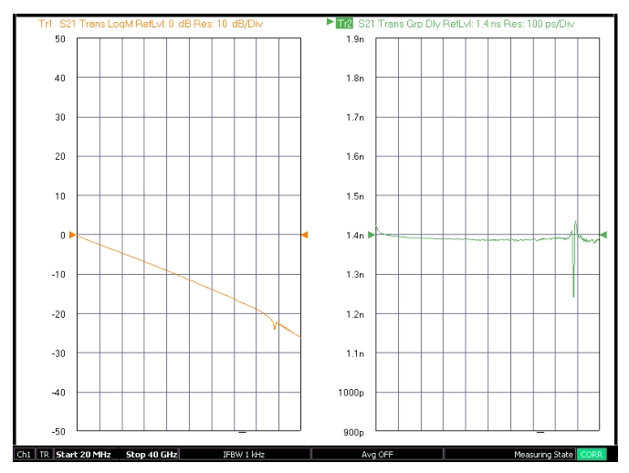
As an example, consider a long PCB transmission line that has a frequency domain S21 like that shown in Figure: Frequency Domain Transmission Response of the Example DUT. A 20 MHz to 40 GHz sweep with 2000 points was used to maintain the harmonic sweep requirement for low pass time domain and eye diagram processing. The loss of this DUT is indeed substantial at high frequencies and there is some additional structure above about 30 GHz. The group delay also shows structure at high frequencies.
Frequency Domain Transmission Response of the Example DUT
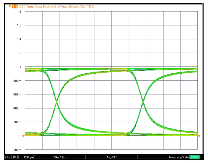
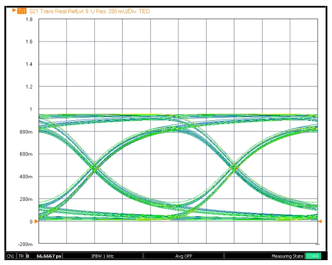
With a 10 GBPS data rate and no assumed jitter, the eye diagram in Figure: Eye Diagram of Example DUT is generated. The eye is still quite open at this data rate.
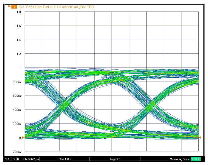
When excited with a 30 GBPS PRBS signal, the eye noticeably degrades further (see Figure: Eye Diagram for Example DUT for 30 GBPS Data Rate). The eye height has reduced from nearly 800 mV to perhaps 600 mV and the rise and fall times as a fraction of the UI have increased further.
Adding 5 ps RMS random jitter, 100 mV RMS AWGN noise and 5 ps rise/fall times (staying at 30 GBPS) further reduces the eye opening but may come closer to predicting a practical environment (see Figure: Eye Diagram for Example DUT for 30 GBPS Data Rate with Higher AWGN Noise and Incident Rise and Fall Times). Because the slewing of the DUT is already so severe, the added rise/fall time effects appear more minor than if the DUT had a less dramatic frequency response.
Eye Diagram for Example DUT for 30 GBPS Data Rate with Higher AWGN Noise and Incident Rise and Fall Times
The 30 GBPS example is repeated but with higher AWGN noise and higher incident rise and fall times.
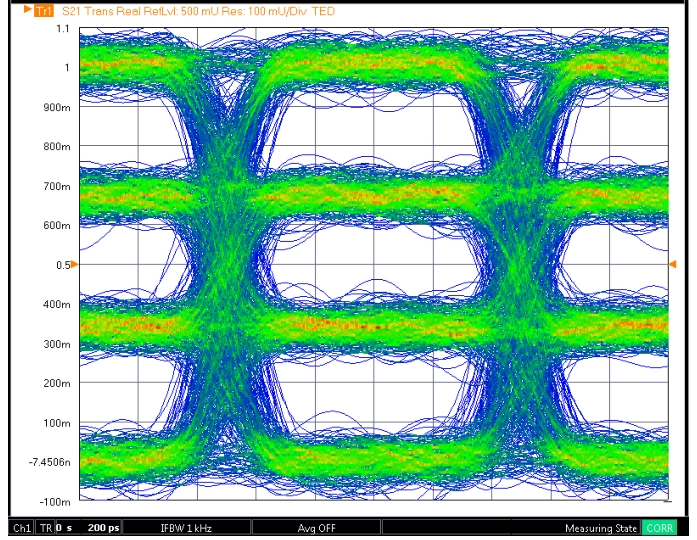
A PAM-4 example is shown in Figure: PAM-4 Example with Added Jitter and AWGN. with relatively high random jitter and AWGN noise. This is a 10 GBPS signal using a 40 MHz-40 GHz sweep range. The default logic levels of 0 V, 333 mV, 667 mV, and 1 V were used. Because of the greater number of possible paths, increased persistence is sometimes used (1000 in this example) to make the display more uniform.
PAM-4 Example with Added Jitter and AWGN.
Eye Diagram Readouts
There are a wide variety of readout values (or eye statistics) that are available. These parameters can be enabled in two groups (vertical-based and horizontal-based) and will appear on the trace graticule much like certain marker search parameters (e.g., resonator Q) discussed elsewhere. These parameters are
• Vertical-based (note these are all on a per-eye basis for PAM-4)
• Logic Levels (0 and 1 for NRZ, four levels for PAM-4)
• Level mean
• Amplitude
• Height
• Signal to noise
• Rise time
• Fall time
• Duty cycle distortion
• Horizontal-based
• Width
• Opening factor
• Jitter (pk-pk and RMS)
As might be gathered from Figure: Generic Eye Diagram Plot, these quantities take on a statistical nature since the data at each point of the eye diagram (in the sense of a slice in the vertical direction or one in the horizontal direction) contains a collection of values. Indeed, the above parameters are evaluated based on histogram-like analyses of the distributions.
Note that this list is separated differently from the amplitude‑based and time‑based separations in the user interface. The above list is based upon how the parameters are calculated, whereas the user interface split is based on how the parameters are typically used. For reference purposes, the user interface items based on amplitude are Logic Level, Level Mean, Amplitude, Height, Opening Factor, and Signal to Noise; and those based on time are Width, Rise Time, Fall Time, Pk-Pk Jitter, RMS Jitter, and Duty Cycle Distortion. For PAM-4, the vertical quantities are analyzed one eye at a time so there are three sets of numbers in each slice.
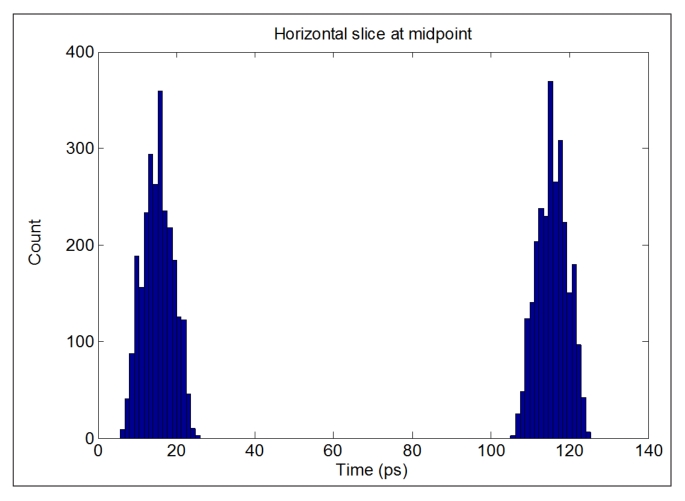
As an example, consider a horizontal slice in the middle of the vertical scale. The histogram of this slice is shown in Figure: Histogram Pertaining to Horizontal Slice Through the Middle of Eye Diagram and shows two distributions at the transition midpoint; one on each side of the eye. The distance between the mean of the two distributions gives an idea of eye width while the standard deviation of one of the distributions gives a measure of jitter.
Histogram Pertaining to Horizontal Slice Through the Middle of Eye Diagram
The histogram pertaining to a horizontal slice through the middle of an eye diagram is shown here. Although mainly for illustrative purposes, the distributions shown help visualize how the eye parameters are calculated.
For the horizontal parameters, these are the definitions used:
• Width: (Right distribution mean—3 ∗ standard deviation of right distribution)—(left distribution mean + 3 ∗ standard deviation of left distribution)
• Pk-Pk Jitter: Absolute width of the distribution
• RMS Jitter: Standard deviation of the distribution
• Duty Cycle Distortion: If the rising and falling edge distribution means separate at the mean amplitude point, this difference (in time or in % of the bit period) is the duty cycle distortion.
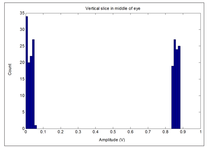
Similarly, a vertical slice, positioned in the middle of the open eye, is shown in Figure: Histogram Corresponding to Vertical Slice Through Middle of an Open Eye. Here the difference between the means of the two distributions gives a measure of eye height while the standard deviation could be used to compute a signal‑to‑noise ratio. The histogram bins were chosen rather randomly for these plots but is the computed statistics that are used for the readout parameters.
Histogram Corresponding to Vertical Slice Through Middle of an Open Eye
Consider first NRZ signaling. For the vertical parameters, these are the definitions used where a slice in the middle of the eye is used:
• 0 level: Mean value of left distribution
• 1 level: Mean value of right distribution
• Level Mean: Mean of all data
• Amplitude: Mean of right distribution—mean of left distribution
• Height: (Mean of right distribution—3 ∗ standard deviation of right distribution)—(mean of left distribution + 3 ∗ standard deviation of left distribution)
• Opening Factor: Ratio of eye height to eye amplitude
• Signal to Noise Ratio: (Eye level 1 – Eye level 0)/ (sigma of left distribution + sigma of right distribution)
Rise and fall time need a sweep through some vertical slices:
• Rise Time: Time from when the mean of the left distribution reaches the set low rise time, e.g. 10%, of the eye amplitude above the eye level 0 (starting from a mean at eye level 0) to the time (after a crossing) when the mean of the right distribution reaches, e.g. 90%, of the eye amplitude above the eye level 0. The low rise time is user-defined, the high fall time is 100% – RiseTime.
• Fall Time: This is the same as above except starting from eye level 1 on the right distribution and working down.
Consider next PAM-4 signaling. The essential quantities are the same as the above, but each eye (thinking vertically) is considered one at a time, so there are three sets of parameters for each slice. The rise time and fall time are bit ambiguous, since different transitions are in play, but the value is computed from the same distributional transfer.
Eye Diagram Limit Lines and Their Configuration
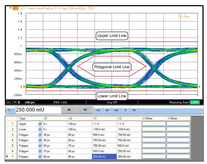
Limit lines are of value in eye diagram measurements just as in other VNA measurements although the topology of those limit lines is somewhat different due to the nature of the data. While traditional ‘upper’ and ‘lower’ limits still are useful and serve to demark limits of overshoot and undershoot, there is now an additional concept of a ‘polygonal’ limit line to constrain the amount of eye closure to be allowed. An example of all three types of allowed limit lines are shown in Figure: Eye Diagram Mode Display and Limit Line Table.
Eye Diagram Mode Display and Limit Line Table
The display and limit line table in the eye diagram mode is shown here with polygonal line items shown. Normally three or more polygon segments are used to form a closed structure. The polygon will automatically be closed if a complete set of segments have not been entered. The segments of the polygon should be entered sequentially (clockwise or counterclockwise) so the system can figure out which region to enclose.
The upper and lower limit lines are covered elsewhere in this guide. The polygonal lines apply only to eye diagrams and that choice in the limit line table only appears in this mode. The polygonal limit line must have at least 3 vertices and must be closed. The system will automatically close the polygon if a complete set of segments have not been entered. The interior of the polygon is always considered the ‘Fail’ zone.
For PAM-4 signaling, there are 3 polygonal limit lines allowed (scanning each of the three eyes stacked vertically) with their own set of independent vertices. Again, at least 3 vertices are needed for each and the polygon must be closed. A limit failure will be indicated for a violation on any min/max line or any of the polygons.
Eye Diagram Recommendations
As with many time domain-based VNA measurements, using the largest frequency domain sweep range possible where the DUT still has a response and is not radiating severely will lead to the most complete time domain response.
In terms of the calibration quality, cable/connector issues most strongly affect the low frequency and wide-ranging phenomena that have the most time domain impact. Paying more attention to those aspects of the setup and calibration process can pay good dividends. The very low frequency response has less of an effect as the data rate approaches a reasonable fraction of the measurement bandwidth. In these cases, the intrinsic rise/fall time starts to dominate the eye shape.
Depending on the level of mismatch involved, a transmission frequency response calibration (or a simple trace memory normalization) may be an adequate level of calibration. A full port calibration will reduce uncertainty and may be required for reasonable eye diagrams if the mismatch levels are high. Any of the VNA’s de-embedding tools may be invoked prior to the eye diagram calculation.
When using jitter and rise/fall time entries, keep in mind that the limits on these scale inversely with the bit rate (as they tend to do in practice).
The eye diagram results are effectively simulations based on frequency domain data of the connected DUT. As such, they may not represent an entire system and they rely on relevant entries for noise, jitter, rise/fall times, and amplitudes.