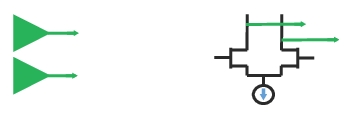
Noise figure definitions present some interesting challenges, particularly in a multiport context. To start, consider the IEEE definition, which is somewhat intrinsically 2-port. It relies on the noise power out of a DUT when the input is terminated, in a reflection-less way, with a body at T0=290K.
Classical Configuration Assumed for 2-port Noise Figure Measurements
The input termination is assumed to be noisy but reflection-less.
Now, as has been discussed in the literature [1], the multiport situation raises some questions:
• Can we segregate ports into ‘input’ and ‘output’ classes?
• How are the input ports terminated? Are all at T0 or are all but one ‘noiseless’? If all are noisy, are those noise signals correlated? Does it matter if the distribution of input noise is by port or by mode?
• If measuring noise at output port M, how is output port N terminated? Can the output port be terminated indirectly (e.g., through a probe) with minimal accuracy impact?
How are noise parameter inputs to be thought of? A vector of input impedances and an input correlation matrix?
Choosing the Noise Figure Definition for a Differential Device
For a differential device (or for a multiport DUT in general), the existing noise figure definitions are somewhat incomplete, but reasonable choices can be made.
The input/output assignment question ends up having little practical impact. For a passive DUT, one can assign these on the fly and for an active DUT, it generally follows logically: those ports that have gain to some other port should be terminated in T0. As we will see later, the passive network case ends up being less confusing than it might seem.
Why should we terminate the inputs in noisy T0 terminations? One could generate a more detailed picture of a DUT by using some noiseless terminations and other combinations, but recall that noise figure is generally intended to represent a simple way (with a single value) of expressing the noise output of a DUT under some representative conditions. The more complete description is left to noise parameters. Practically speaking, it would be hard to apply noiseless terminations to certain ports for measurement and would not represent many practical use cases anyway. Extending the 2-port definition makes sense in this way. The next question is one of correlation of the inputs (and there will be much more on this later): should the input noise sources be uncorrelated or correlated in some manner? Going back to noise figure-as-a-single-number concept, it would seem to make sense to have the inputs be uncorrelated since (a) that is practical from a measurement perspective, (b) it is the most easily described configuration, and (c) the correlated case is best handled in the realm of noise parameters since there is an arbitrarily large number of possible correlated inputs.
The output port terminations again go back to the question of assignment. In the case of a device with gain, the terminations on the output ports not being measured are going to have little practical impact (assuming the DUT doesn't oscillate in this case.). In the case of a passive network, all ports not being measured should be assigned the state of 'input' and be appropriately terminated for the definitions to be consistent.
Before going further, it may be helpful to revisit the concept of correlation. Mathematically, the cross-correlation of two signals is simply (where * denotes complex conjugate)
Equation 20‑6.
Where N is some positional index that might reveal some information when two signals are related but shifted relative to each other. In general, if b1 and b2 are noise signals from independent sources (and have zero mean), one would expect this sum to be very small in the limit of many samples since each individual b1b2 product will be randomly phased. If, however, the two noise signals are derived from the same source, there would tend to be some common phase relationship between b1 and b2, so the product terms will all tend to align and the sum becomes non-zero. This is the result for two correlated noise signals.
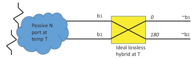
Consider next a passive network (with T-terminated inputs) at temperature T. Ignore all reflections and connect an ideal, lossless hybrid at the output so we have some final output signals ~b1 and ~b2. This line of analysis was reported in [2].
Noise Correlation Behavior in Passive Multiport at Thermal Equilibrium
A measurement thought experiment (after [2]) is sketched here to illustrate noise correlation behavior in a passive multiport at thermal equilibrium.
Because everything is at temperature T (and is presumably at equilibrium), the noise powers in the various output places must be the same and equal to kTB where k is Boltzmann's constant and B is the measurement bandwidth.
The only way both equations Eq. 20‑8 can be true is if =0. But this is just the real projection of correlation. If we repeat this thought experiment with a 90 degree hybrid instead of a 180 degree hybrid, we will reach the conclusion that =0. This interesting result (called Bosma’s theorem) is that noise power emanating from a passive multiport must be uncorrelated. Not only does this lend some further justification to our noise figure definition, but it also makes it practically much easier to analyze the effects of network losses before the DUT (probes, pads, etc.): they do not induce any input correlation.
In terms of an actual active DUT noise figure measurements, what are then the impacts of correlation? On one level are the users’ system implications: how will the DUT outputs be used? If they end up feeding single-ended receivers, it may not matter much. If they feed another stage in a fully differential system, it may matter quite a lot. In terms of the DUT outputs themselves, the degree of correlation has much to do with the internal topology of the device. While the analysis cannot be exhaustive here, one can consider two extremes. Suppose a packaged differential amplifier has noise dominant stages that are actually separate single-ended amplifiers (left side of Figure: DUT Topology Influences Correlation of Noise Power Between Output Ports). Assuming the dominant noise source within those stages is not some shared bias system, it is quite likely that the output noise will not be highly correlated.
DUT Topology Influences Correlation of Noise Power Between Output Ports
DUT topology has a large influence on the correlation of noise power between output ports. Separate dominant gain stages could make correlation negligible, but a dominant differential pair would do the opposite.
If, however, the dominant noise source is an output differential pair with much of the noise derived from a common source bias (right side of Figure: DUT Topology Influences Correlation of Noise Power Between Output Ports), then the output noise will likely be highly correlated. Depending on one’s knowledge of the DUT structure, it may be desirable to choose a measurement method that fits most closely. If not much is known, then doing the additional work to ensure correlation is treated correctly may be useful.


 =0. But this is just the real projection of correlation. If we repeat this thought experiment with a 90 degree hybrid instead of a 180 degree hybrid, we will reach the conclusion that
  =0. This interesting result (called Bosma’s theorem) is that noise power emanating from a passive multiport must be uncorrelated. Not only does this lend some further justification to our noise figure definition, but it also makes it practically much easier to analyze the effects of network losses before the DUT (probes, pads, etc.): they do not induce any input correlation.