Since at its core, a noise figure measurement discussed in this chapter is a combination of a noise power measurement and analysis of DUT gain, many of the uncertainty components are the same as for single-ended noise figure. As discussed in Noise Figure (Option 41), some of these elements are:
• Accuracy of DUT gain. This is an S-parameter uncertainty problem, but in this chapter it may involve those derived from 4-port measurements. The contributing factors are the same and the S-parameter uncertainties are discussed in great length elsewhere.
• Power calibration and receiver calibration accuracy. Since a cold source method is used for the differential noise figure measurements as well, how the power reference plane is established matters.
• System noise floor and having adequate gain (and noise figure) in the DUT and composite receiver is essential to getting the noise power in a linear range for the VNA analog-to-digital converters.
• Sufficient RMS points per frequency to keep measurement jitter tolerable.
Specifically for differential noise figure (aside from the slightly different gain computations and different net uncertainties in those terms), there is the context of the measurement that is important: defined with uncorrelated noise inputs at temperature T0 and all terminations are reflection-less. While not that different from the 2-port assumptions, there are more places for changes to happen in the setup. There is then the topic of correlation between DUT outputs that has been a central topic in this chapter. Balun-based Methods and Handling of Imperfections showed the scale of errors in neglecting correlation in balun (combiner)-based methods and there is an uncertainty contribution from the S-parameter measurements of the balun. In the case of the direct correlation method, there is an S-parameter-like term embedded in the correlation calibration (how accurately can the phase reference plane be established, which will be affected by port match, etc.) and from the ability to correct for receiver-network-induced de-correlation (which will depend on relative gain levels and electrical length differences).
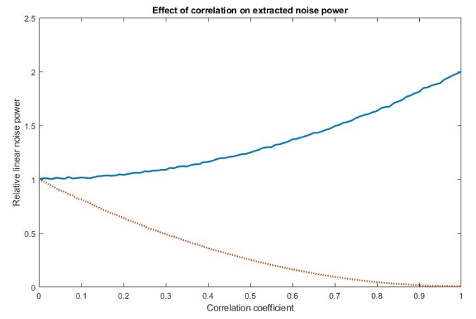
More generally, the effect can be somewhat self-evident by looking at Eq. 20‑10. Using arbitrary scaling, suppose the average of single-ended noise powers was 1 linear unit. If the DUT outputs are completely uncorrelated, the common-mode and differential noise powers will also be 1 linear unit. At the limit of full correlation, they could reach values of 0 and 2, respectively (or the other way around for a common-mode amplifier) so the percentage or dB errors can be extreme, theoretically. In practice, this is usually not the case (and, indeed, often one does not care as much about common-mode noise figure since the gains are so low; there are also additional uncertainty complications with the lower noise power since the subtraction of nearly equal numbers is involved) but the potential errors may be useful to understand.
Monte-Carlo Simulation of Extracted Noise Powers for Different Levels of Correlation
A Monte-Carlo simulation of extracted noise powers for different levels of correlation for the differential (blue/top)) and common-modes (red/bottom), assuming a differential amplifier. The end points of the curves are easy to understand on an ideal level.