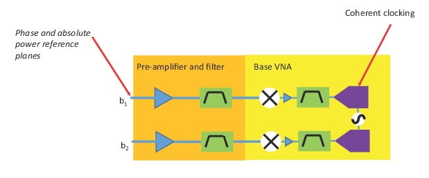
Another method can take advantage of having multiple, time-coherent, IF channels in the VNA to get at correlation between DUT output ports directly. Since the noise waveforms are directly digitized after IF processing, correlation between two noise signals can be maintained after certain levels of correction. This is the principle illustrated in Figure: Correlated Noise Measurement Example Showing Coherent Digitizers.
Correlated Noise Measurement Example Showing Coherent Digitizers
In correlated noise measurements, the external hardware configuration is largely the same (see text) but coherent digitizers in the instrument are used to help directly identify the correlation levels.
If the correlation is directly measurable, then the differential and common-mode noise powers are
Equation 20‑10.
Of course, there are complications:
• The b1 and b2 measurements are now complex quantities, so a phase consistent reference plane must be established. The correlation calibration was established to achieve this using ratioed measurements against a deterministic signal from an internal source. A thru line connection to each receiver path is all that is required, and this can be done at the same time as a receiver calibration. As with the receiver calibration, the system will interpolate/ (flat-line) extrapolate if the frequency range is different at measurement time vs. calibration time.
• At some point in a setup, coherence time can come into play. That is, two noise signals will only retain their coherence relative to each other over some finite length of line (even if well-matched). This is not necessarily intuitive, but is demonstrated in a more obvious way with the famous Michelson-Morely experiment (e.g., [8]) when performed with white light. In this experiment, two paths of different electrical lengths are made to interfere and create interference fringes. When the lengths get longer, these fringes get less distinct and eventually vanish when using broadband, white light. The concept is that every source has some inherent coherence time that scales as 1/ (bandwidth) that describes the scale over which this occurs. For a VNA noise measurement, the bandwidth of relevance is the IF bandwidth of the measurement system, which is of order 1 MHz or smaller, so the length scales that could be a concern are longer than 1 microsecond.
• Even aside from coherence time, the receiver network itself can de-correlate a pair of incoming correlated noise signals. If the gain and noise generation of the receiver system greatly exceeds that of the DUT, the uncorrelated noise of the receiver system (assuming distinct amplifiers are being used) could wash out the signal correlation, and this cannot be recovered. Although good practice, as discussed in Noise Figure (Option 41), the receiver pre-amplifier chain should have just enough gain to pull the kTB base signal out of the instrument floor. In addition, radically different electrical lengths of the receiver chains can de-correlate the signals in a periodic fashion, but the instrument uses the frequency response of the correlator calibration functions to partially correct for this. This correction relies on the frequency sweep being sufficiently wide relative to the electrical length delta, so adding some asymmetry to the setup is helpful for narrowband devices. If a CW frequency is being measured (or the frequency sweep is extremely narrow relative to the electrical length difference), a different algorithm will automatically activate that de-embeds receiver network correlation effects, but accuracy is reduced, mainly for the non-dominant mode (e.g., common-mode noise power for a differential amplifier will have reduced accuracy).
• Because of the use of frequency relationships, the data only updates at the end of sweep when in this mode.
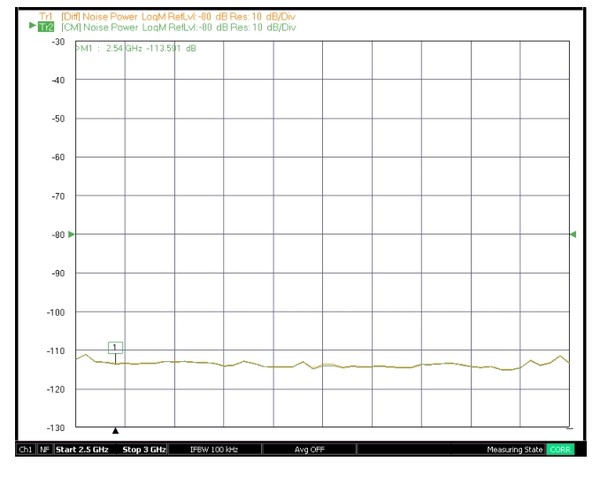
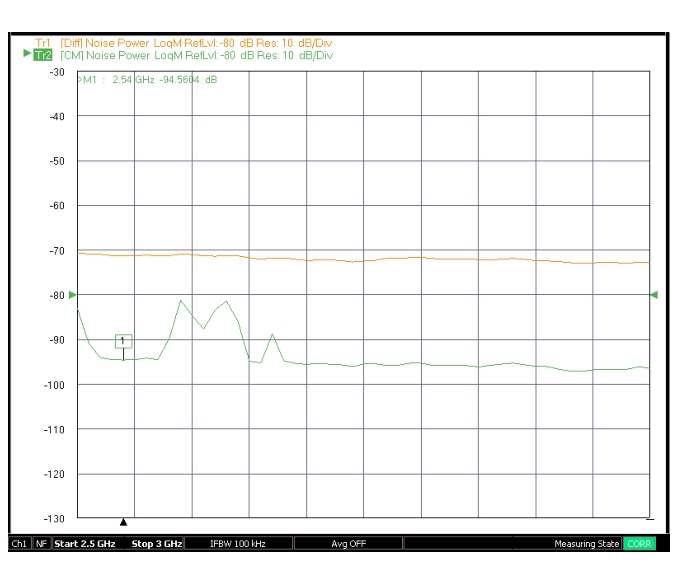
As an example, consider the noise power from a passive DUT. From the earlier discussion, one would expect these to be uncorrelated and, in this measurement example, the differential and common-mode noise powers do essentially overlay (see the example in Figure: Correlated Noise Measurements Example for Passive DUT). When a differential amplifier is measured (whose internal topology suggested a fair amount of noise correlation was likely), a very different result is obtained, as shown in Figure: Correlated Noise Measurements for Differential Amplifier. Here the differential mode noise power exceeds the common-mode noise power by at least 10 dB (and by >20 dB at some frequencies). There is a lower limit to the correlated power measurement, set by the single-ended floor, so soft clipping will result in some measurements. In this particular case, the common mode output impedance was such that even the thermal noise contribution to this mode was small at many frequencies.
Correlated Noise Measurements Example for Passive DUT
• Perform a power calibration on port 1 (if desired) at a sufficiently low level that the composite receivers will not compress. Perform a receiver calibration (using this power calibration, if desired) and correlation calibrations on both receiver paths (the receiver and correlation calibrations can be done simultaneously using the checkbox in the CALIBRATION dialog. These calibrations can be done while in the noise figure application or can be recalled.
• Perform a noise calibration on both receiver paths with terminations attached to the receiver inputs.
• Load DUT S-parameter or gain data.
• Connect DUT and measure.
The steps are essentially the same as in Figure: General Calibration and Measurement Steps (part 1)., since the receiver and correlation calibrations can be done with the same connection. A checkbox in the CALIBRATION dialog allows the two calibrations to execute simultaneously.