Final topics for this chapter cover some ancillary measurements, including:

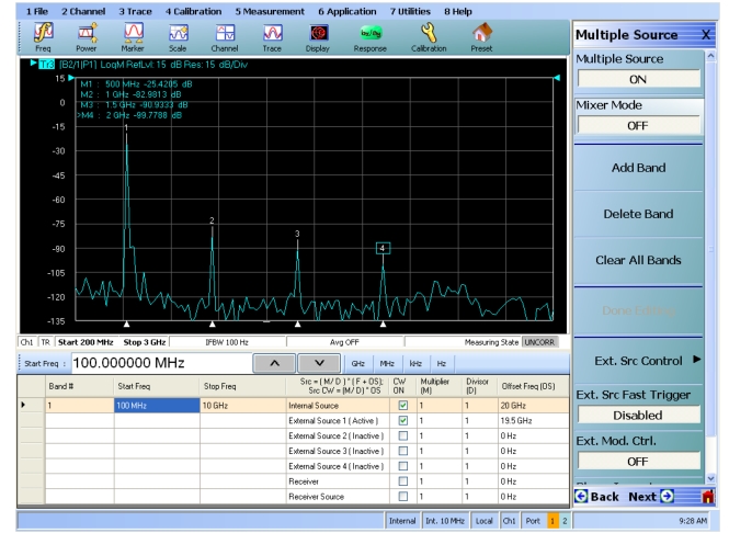
The MS464xB can be used as a spectrum monitor to scan for spurious products of the mixer. This is most easily done with multiple source control (see Multiple Source Control (Option 7)) with the input source and LO usually set to some CW frequencies and the receiver allowed to sweep over a range of interest to look for spurious products on the LO. The unratioed test channel is often used as a monitor and a receiver calibration can be applied to get an absolute signal level for those spurious products. An example setup is shown in Figure: Multiple Source Setup—Search for Spurious Products where the source is parked at 20 GHz and LO at 19.5GHz. The desired IF is 0.5 GHz but we can sweep over a wider range to look for products and the result is shown in the figure as well.

In this particular case (and with the sweep resolution used here), the dominant spurs are all harmonics of the IF. Using the previous nomenclature, they are of the form N × (Input – LO) and they are all at least 55 dB below the desired IF. With a different sweep range and point density, other spurs might have been found so it does help to work out the frequency plan in advance where likely spurs might reside.

One does have to exercise some caution in interpreting these results since the VNA receiver is not pre-selected and there may be internally generated spurs as well. In addition, the internal converters have an image located (usually) 24.7 MHz above the programmed frequency (at certain frequencies below 50 MHz, the offset is slightly larger). It usually pays to back calculate the product orders to see if they make sense for the DUT’s frequency plan.

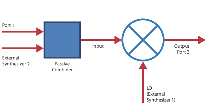
Using multiple source control again and two external synthesizers, it is quite easy to configure an IMD measurement. The measurement concept is covered in more detail elsewhere but the basic idea is to apply two closely spaced sinusoids to the input of the DUT (at frequency f1 and f2) and examine the third order products at the output as shown in Eq. 21‑3 below:

The setup is shown in Figure: Mixer Setup for IMD Measurement and the multiple source configuration is shown in Figure: Example of Multiple Source Setup For CW Mixer IMD Measurement below.

Typically b2/1 is the response variable and the measurement can be constructed to be CW (to look like a spectrum analyzer output) or swept to reveal the IMD product magnitude vs. frequency (in either dBc or dBm terms). The CW-measurement is illustrated in Figure: Mixer Setup for IMD Measurement below where the sources are kept fixed and the receiver is allowed to move over the range of interest.

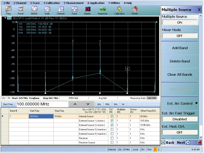
A segmented sweep setup was used in Figure: Example of Multiple Source Setup For CW Mixer IMD Measurement with 11 points (spaced by 200 kHz in this case) around the main tones (a 50 MHz tone offset was chosen), the 3rd order products and the 5th order products. This can optimize measurement time by not measuring frequencies that are not of interest and it allows one to measure quickly when at the main tones (large signals) and in a narrower IFBW when measuring the products (since they may be close to the noise floor). External synthesizer 2 was used to create the 2nd tone and its amplitude was adjusted to make the main tone levels approximately equal although other values could be chosen. In this example, the upper and lower products are not symmetric which may be an indication of bias network interaction within the DUT, compressive behavior in parts of the DUT, or other memory effects.

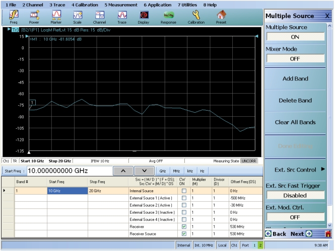
The swept measurement is shown in Figure: Example of Swept Mixer IMD Measurement where the LO is fixed but the two source-like synthesizers are sweeping along with the receiver. In this case the tone offset was chosen to be 30 MHz. The only practical limit (outside of DUT bandwidth) is that very small offsets may incur a noise penalty and the synthesizer noise skirts start to interact. This normally does not happen until below 1 MHz offset depending on the synthesizers being used. The receiver is kept locked onto the upper IMD product in this case. Here just a receiver calibration was used so the readout is the product in absolute power terms (dBm). By doing a sweep with the receiver at a main tone (470 or 500 MHz in this case) and doing a trace(/)memory normalization, one could then measure the product in relative (dBc) terms.

While the ‘modular BB’ check box in the mixer wizard was discussed earlier in this chapter, some additional information on setting up mixer measurements in the higher frequency bands may be helpful. As stated before, the mixer setup assistants are really configured for fundamental mixing while multiple source control is used directly for more complex cases. Many millimeter wave converting DUTs are harmonic converters, so by nature one will use the multiple source path more often, but we can discuss the use of the assistants.

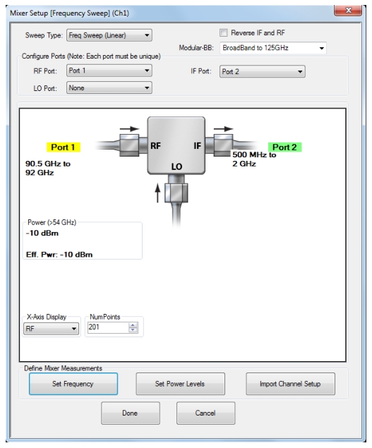
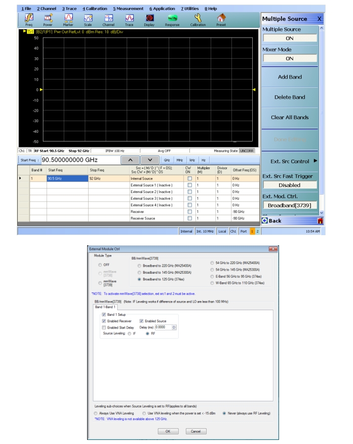
The checkbox in the wizard/setup aid allow the frequency ranges to enter the millimeter wave band and will properly configure the system for the use of the mmWave modules. As an example, consider a W-band mixer with a fixed external LO at 90 GHz and the desire to run the RF over 90.5-92.0 GHz with a 0.5-2.0 GHz IF. The active channel mixer dialog is set up as shown in Figure: Active Channel Mixer Setup Dialog for a Millimeter Wave Example, where no LO was selected since it is external and uncontrolled. One can then look at the multiple source setups (Figure: Resulting Multiple Source Screens for the mmWave Mixer Setup Example). Most importantly, the external module control dialog has been activated.

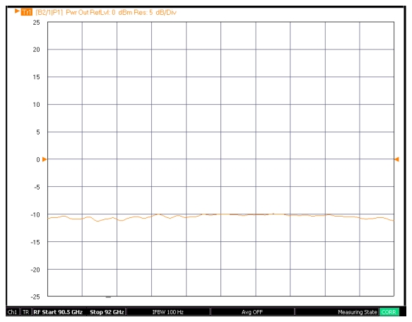
The same calibration protocols as before are available for the modular mmWave modules. For this particular DUT, a normalization calibration was performed and the resulting conversion loss measurement is shown in Figure: Example Millimeter Wave Conversion Loss Measurement. Prior to entering the mixer mode, a user power calibration was performed on the mmWave module as discussed in Broadband/mmWave Measurements (Option 7, Option 8x). This accuracy transfer is important to the overall uncertainty.

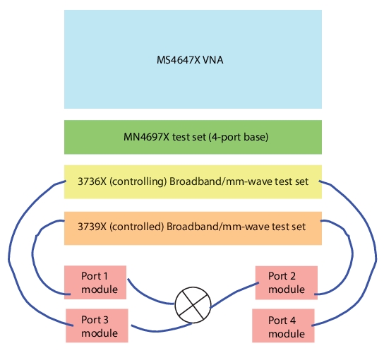
Even with dual sources, it is not possible to use both internal sources (i.e., both input and LO) for an active mixer broadband setup. It is possible to set this up manually with multiple source control. With a 4 port, dual source broadband/mmWave system, however, it is possible to set this up directly with both active channel and multi-channel tools. To keep the choices manageable, the input and output are restricted to be amongst ports 1 and 2 ('none' and external sources can be still be selected for the input) and the LO can be either port 3 or port 4 ('none' and external sources are still possibilities). An example setup is shown Figure: Example 4-Port Dual Source Setup.

For higher millimeter wave bands, multiple source alone is the setup choice because of the complex frequency plans that are involved.

For mixer measurements in general, but particularly mmWave mixer measurements, power calibration is an important accuracy aspect as has been discussed. Since millimeter wave signal generation sometimes does not have as high a level of harmonic and sub-harmonic filtering, there can be differences between integrated power (that a power sensor measures) and fundamental power (that a VNA measures). As the harmonic content levels rise, this can lead to inaccuracies when basing a VNA measurement on a power meter calibration. For the modular broadband/mmWave case, the user power calibrations in VectorStar have an available fundamental power correction (checkbox available on the user power calibration dialog) that helps to reduce this problem by using measurements with the VNA receivers to estimate harmonic content instantaneously during the calibration and correcting the power targets accordingly. More information is available in Fundamental Power Correction located in Multiple Source Control Set Up of this guide.