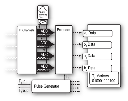
To explore the high-speed digitizer method in more depth, consider the acquisition system of the Anritsu MS4640B with Options 35 and 42 shown in Figure: Block Diagram: Acquisition System in the MS464xB Series with Option 35 and Option 42.

Details on the functionality and performance of the IF digitizer are covered in this section.

IF signals are generated by the down converters in the MS464xB Series. When equipped with Options 35 and 042, the standard IF system is bypassed, and signals are routed to a special high-speed digitizing IF board. This board consists of analog processing (filtering, gain, calibration and other factors) in a much wider bandwidth than the standard IF system to enable the measurement of much narrower pulses. This board also houses the fast analog-to-digital converters, the pulse generators, and digital processing components.

A large block of configured memory is used to store the data from the converters. This data is keyed with the T0 synch information. For the pulse measurement processing, the data of interest is selected (relative to T0) and run through the appropriate conversions to the frequency domain. S‑parameters are then created and the appropriate calibrations are applied.

Since the processing is relative to these time markers and not any of the pulses per se, there is considerable flexibility on where in time one can look at the results. This flexibility becomes particularly valuable in complex pulse situations where many sub-pulses are present or when multiple external generators are being used.

Narrow pulses and fast edges can be captured with a minimum resolution of about 2.5 ns. Since the memory is very deep, very low duty cycles and low repetition rates are supported without sacrificing resolution. For pulse repetition rates in the Hz range and slower repetition rates, normal triggered methods are sufficient.

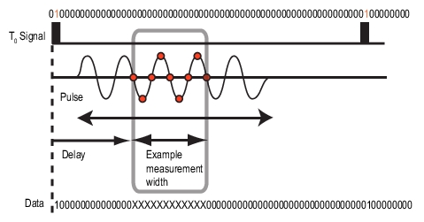
From the point-of-view of the measurement, normally only the delay (or delay and the number of measurement points for pulse profiling) and measurement acquisition width must be specified. To further understand the acquisition process, consider the point-in-pulse measurement shown in Figure: Using Acquired Data from a Pulse-to-pulse Measurement. In these cases, the data of interest (denoted with x's) begins at some number of samples (delay) after the T0 edge.

The time domain data is converted into a single frequency domain point. If a smaller width had been entered, fewer samples would have been taken. In this way, the measurement width acts as an effective processing bandwidth (for example, an IFBW).

This result can be averaged over multiple pulses to reduce trace noise or increase effective dynamic range. In this case, the x's will be collected after multiple T0 high markers until the desired level of averaging is complete.

During the acquisition, pulse timing is coherent with the ADC clock to maintain phase. It is presumed, in the election to perform a point-in-pulse measurement, that the DUT response is consistent over multiple pulses (or that the goal is to average that behavior). The total acquisition time is computed based on the requested averaging and the PRI. If one wants to look at more individual pulse behavior, then the pulse-to-pulse measurement mode is recommended.

Pulse-to-pulse and pulse profiling measurements are processed in similar ways. For pulse profiling, a single acquisition is completed (based on time span of interest, PRI, and requested averaging). That data is sequentially processed using the selected measurement width at each of the requested time points. If averaging is enabled, the process is repeated over multiple pulses. In the pulse-to-pulse measurement mode, the data is acquired over the measurement width requested, and then the same measurement window is processed separately per period.

To understand the number of pulses that must be acquired, consider an effective IFBW (=IFBW/(pt-pt averages)….sweep-by-sweep averages are handled as a post-processing task). If this value is larger than 1/(measurement window) then only one pulse is needed although two may be acquired to guarantee synchronization. As the request IFBW shrinks, addition pulses will be captured for point-in-pulse and pulse-profiling measurements.

For example, given the following parameters:

Effective IFBW is 20 kHz, so acquisition over 50 pulses will be required (with potentially an additional pulse to guarantee synchronization).

The measurement resolution in pulse mode is set by the ADC clock rate and generally defaults to ~2.5 ns (except for receiver frequencies < 110 MHz). This in turn puts a lower limit on measurement width. This also sets the maximum acquisition length which in turn limits the maximum PRI. Without Option 36, the maximum acquisition length at the default resolution is 0.5 seconds and the maximum PRI is 0.25 seconds (these values scale proportionately for wider resolutions, that is, slower ADC sampling rates). With Option 36 installed, the maximum acquisition length at default resolution is 2.5 seconds and the maximum PRI is 1 second (these also scale with resolution).

The resolution time can be increased on the PulseView menu up to 90 ns when fine time resolution is not needed but longer acquisition length is desired. The available acquisition length scales proportionately with the resolution entry as do the other pulse parameters.