Pulse profiling measurements are often of interest when changes in performance within the pulse duration may occur. Examples include thermal and trapping time constants or leading edge phase overshoot/undershoot and trailing droop behavior of a pulse phased array module.
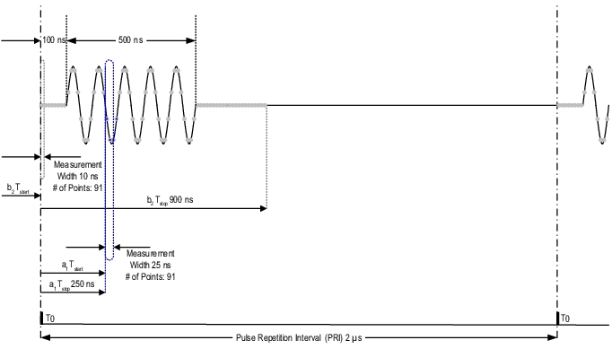
For this example measurement, the PRI is 2 μs and the combined bias/RF pulse width is 500 ns. The goal is to examine the pulsed S21 response using a sliding 25 ns profiling window beginning just before the main pulse and ending just after it.
We are interested in S21, but wish to look at the off ratio as well, so only b2 will be profiled. The reference a1 data will be acquired from a 25 ns window in the middle of the pulse. In order to properly calculate the ratio b2/a1, the profiling point counts have to match although the a1 'profiler' is not moving (this requires that the measurement channels be uncoupled).
A point count of 91 is chosen for this example, making each of the profiling windows non-overlapping (this is not required). Sweep-by-sweep averaging over 10 pulses is used to improve trace noise. With an IFBW of 1 MHz and a profiling width of 10 ns, about 100 pulses-per-sweep are used to compute the result.
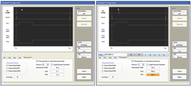
Internal synchronization is being used so that the VNA's internal pulse generators are providing the synchronization pulse for any external generators that might be needed in a larger setup. The PulseView™ Configuration dialog box (Figure: Pulse Profiling Measurement Configuration Showing Different Receiver Configurations) shows two different receiver configurations.
Determining the profiling time range for this measurement is an important consideration. A profiling time in the range of 50 ns to 650 ns might seem adequate, but in setups for this range, important information about profiling could be missed at the end of the measurement.
Note
Consider internal latency of the stimulus modulation (about 35 ns) as well as the delay through the DUT and any cables (about 50 ns in this case).
The action in this example measurement does not start until about 175 ns and does not finish until about 675 ns. Using a larger time span can ensure all of the information is captured and only adds a very small amount to the measurement time.
Pulse Profiling Measurement Configuration Showing Different Receiver Configurations
The measurement trace (top line in the dialog box of Figure: Pulse Profiling Measurement Configuration Showing Different Receiver Configurations) is labeled (on the left side) with the active path to which it corresponds (b2 in this example) and the type of measurement (Profile in this example). It also indicates the span of the profile that has been requested (designated with triangle delimiters) and the profiling measurement width, and it indicates the measurement timing for the active path (b2 in this case).
By selecting the Pulse generators on only during measurement checkbox, the pulse generators will only start up when making a measurement, thus avoiding early device stimulation (the user may be looking at long thermal time constant effects) and some potential overshoot conditions (from level dip release). This feature is available only in pulse profile measurement mode.
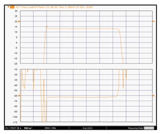
A fast phase overshoot is noted along with a slow gain decay. Only trace normalization (data-divided-by-memory) was used for this measurement.
When examining the pulse edge timing, keep these points in mind:
• All of the delays are referenced to the leading edge of the synch pulse T0,and are defined to the leading edge of the pulse being measured.
• Internally, the mapping of the T0 edge onto the data stream will be correct to within one sample (2.5 ns). When an external T0 is being used, the mapping will normally be correct to within two samples.
• While the pulse edges will be very accurate with regards to the pulse generator output, latency from what these edges drive (the Anritsu pulse modulator test set, other RF modulators, bias systems) can radically change the physical pulses, hence the data interpretation. With a typical cable setup, the latency with the Anritsu pulse modulator test set is around 35 ns. These latencies are normally consistent from test to test. Once latencies are known for a given setup, the results should be interpretable fairly easily. If the setup contains a re-latching or resynchronizing process, there may be a random component to the latency period.