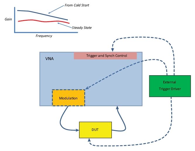
While the PIP measurements discussed earlier in this chapter may be adequate for many swept pulse measurements, there are cases, particularly related to DUT transient response, where more detailed control of the VNA sweep operation relative to the pulses and the measurements is required. This is the purpose of the Continuous Point-in-Pulse mode (CPIP) where the entire sweep of frequency or power is done during one acquisition. A use-case is shown in Figure: Example Use Case of CPIP.

The DUT may operate in a low duty cycle sense (either operationally or for thermal reasons) and then is required to operate over some frequency or power range as in a wide chirp sweep or a quick dynamic analysis sweep. How that DUT behaves during that sweep process may be very different from that when it had been operating steady state (if it could run steady state at all). The inset plot in Figure: Example Use Case of CPIP shows an example of how such a DUT might behave under these two kinds of conditions. CPIP is designed to let one analyze the sweep response from almost any initial condition.

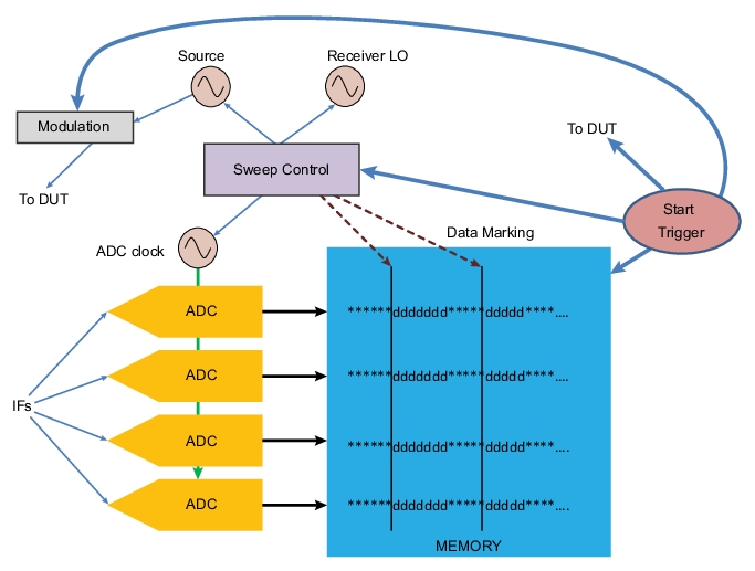
The concept is shown in more detail in Figure: High-level Block Diagram Indicating the Marking Process for CPIP. Since the sweep is occurring during the acquisition, the digitizer memory will be loaded with blocks of data (denoted by the ds in the figure) each corresponding to a different sweep point. There will be (usually small) areas of disrupted data between those blocks where the system is changing frequency or power but the data can be “marked” (as in the external sync marking discussion earlier in this chapter) when the system is stable and the data can be analyzed from that point in the data record (or some controlled amount of delay after that).

Another key point is the triggering of the sweep since the DUT start‑up transients may be great importance. Only per-sweep, per-channel and all-channel external triggering variations are allowed in this mode and the external trigger signal can be used to start the sweep, start the pulse generators and potentially bias/activate the DUT at the same time acquisition begins. Thus a controlled static starting state of the DUT and of the system is a possibility.

An important question is how does the acquisition get synchronized with the sweep? There are two main user‑selectable sub-modes:

An explicit synchronization signal is used in this case and a cable must be connected from the Trigger Out port on the VNA’s rear panel to the Ext Synch In port (also on the rear panel). This provides the most reliable synchronization since the Trigger Out port knows about vagaries in the sweep timing (from bandswitch delays that the instrument requires, slow locking periods, etc.) and adjusts the marks in the data stream accordingly. The Trigger Out and Ext Synch In ports are required in this mode and cannot be used for other purposes.

This is a less explicit synchronization mode and does not require external connections. In this case, the acquisition system has less precise information about the sweep location so it is best suited to narrowband sweeps (not crossing bandswitch points for example) and for slower sweeps where the delay is much larger than the settling time.

In both cases, the sweep rate is set by the PRI (one pulse per sweep point unless burst is used) and the sweep timing is harmonized internally with that PRI. In Synch mode, PRIs as low as 100 μs to 200 μs are possible whereas in Time mode, PRIs of at least 5 ms are recommended (and at least 20 ms if bandswitch frequencies are crossed). As a reference, the common bandswitch frequencies are 2.5 GHz, 5 GHz, 10 GHz, 20 GHz, and 40 GHz (add 38 GHz for 50 GHz and 70 GHz systems; add 54 GHz, 80 GHz, 110 GHz, and 120 GHz for ME7838A/AX systems; add 54 GHz, 80 GHz, 110 GHz and 130 GHz for ME7838D systems). The maximum pulse widths that are practical scale with PRI. The minimum pulse width is not technically restrained beyond the system 5 ns limit. Narrow pulse measurements very close to the synch mark (i.e., low delay) may be difficult due to post-synchronization settling but may be fine for larger delays. The recommended delay (measurement and pulse) varies with frequency and power settings but at least 10 μs for power levels above ~ –12 dBm and at least 50 μs for power levels of –20 dBm and below are common (ALC final settling times are faster at higher power levels).

While there are no strict point count limits, the total acquisition time is still limited by the memory on the digitizer board (0.5 s for the standard 2 GB of memory at the default resolution near 2.5 ns, 2.5 s with Option 36 installed). Thus if 1 ms is the PRI, ~ 499 sweep points are possible for 2 GB of memory at a ~2.5 ns resolution.

The acquisition length defaults to Number of Sweep Points * PRI but this can be adjusted (usually longer) if the triggering mode being used is adding inconsistent delays, or if there are related problems where the last few sweep points show drop‑outs. If the synchronization marks are not received within the acquisition length, the output wave variables will be assigned the value –400 dB.

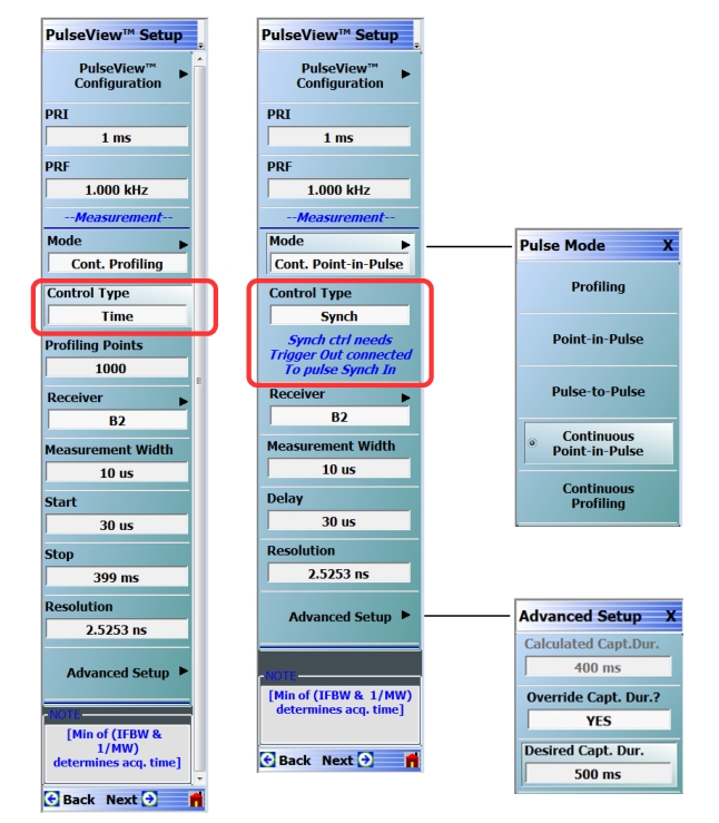
A few highlights of the menu choices when in this mode are pointed out in Figure: Control Type Becomes Available in CPIP and in CProf Modes. The control type (Time or Synch) becomes available in CPIP (and in continuous profiling mode, or CProf, as will be discussed). Also the Advanced Setup button which leads to a submenu for entering acquisition length override and values becomes available.

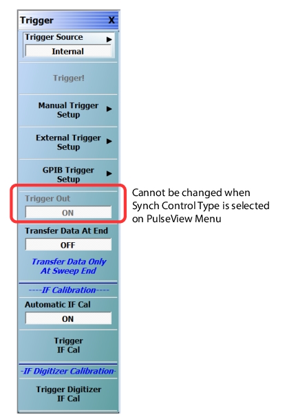
When the Synch control mode is chosen, one would note on the Trigger menu that Trigger Out has been put into the ON state and cannot be changed (Figure: Trigger Menu when in CPIP Mode with Synch Selected). This would not be the case for the Time control mode.

As with the other pulse modes, user calibrations should be performed in this mode for measurements in this mode. All of the calibrations available for PIP are available for CPIP (frequency response, 1-port, 1 path‑2‑port, full 2-port calibrations, all 3-port and 4-port calibration variations, receiver and power calibrations, etc.) Since the sweep dynamics and measurement profiles are quite different, calibrations cannot be shared between PIP and CPIP. Note that measurements and calibrations are still indexed with frequency or power, respectively, and not time since each measurement is still associated with a sweep point.

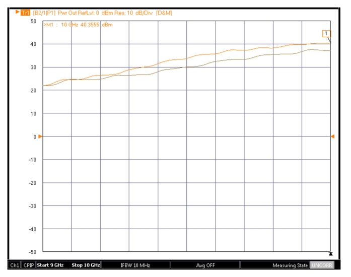
One example measurement is shown in Figure: Example Measurement of DUT Output Power vs. Frequency. We are interested in the device output power vs. frequency and the plot shows both the steady state PIP response (lower trace) and CPIP response (upper trace). In the steady‑state response, there is some power reduction, presumably from heating, at the higher power levels available at higher frequency. This is one example where the DUT dynamics can convolve with the frequency or power response to produce an entirely different measurement result. By performing the measurement under the actual time‑sequence‑of‑events that is of interest, a better understanding can sometimes be achieved.

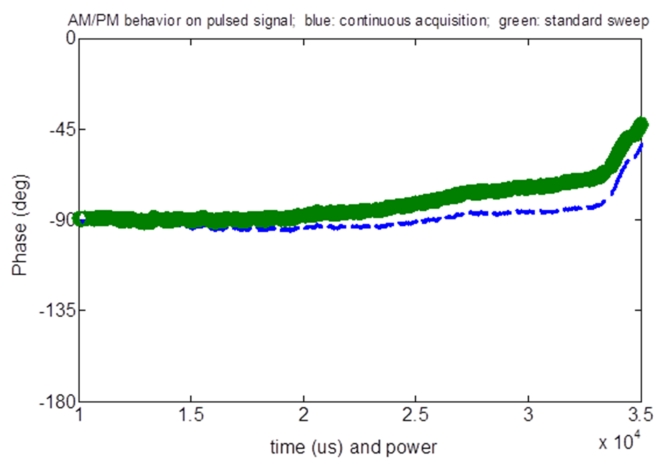
A second example is shown in Figure: Example CPIP AM/PM Measurement and involves an AM/PM measurement of a device. Here the power is sweeping from –20 dBm to 0 dBm over 35 ms and is plotted externally in time in order to give another vantage point. When measured with a standard PIP sweep (thick green trace), there is a general phase growth and a slight uptick at higher power levels. With the CPIP sweep (dashed blue trace), the lower phase growth is much reduced, from a different thermal and bias timing, and the high power growth is much more distinct.