The Continuous Profiling (CProf) measurement also uses a single acquisition for an entire frequency or power sweep but is a generalization in data analysis relative to CPIP. In CProf, one is not restricted to a measurement window associated with each sweep point but one can have up to 25000 measurement windows dispersed over the entire sweep time or located in some subset of that range. The number of displayed points is equal to the number of measurement windows employed. The acquisition length is limited by memory again so the sweep point count * PRI is capped just as in CPIP but here the number of analysis points is an independent concept.

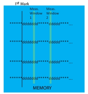
The central idea is sketched in Figure: Measurement Window Positioning in CProf where the sweep starts as in CPIP with a data mark. In CProf, the measurement windows are specified with the familiar start delay, stop delay, measurement width and number of analysis points. In the figure, only the first two measurement windows are shown but they are positioned relative to just the first sync mark when the sweep began. This gives the user considerable flexibility on where to look at data (in time) within each sweep point.

The higher level description of the application for the CProf measurement is similar to that for CPIP but where the requirement is for greater flexibility in looking at the data in time. As such, this measurement approach has applications for many time‑running setups including antenna rotation/antenna pattern investigation, evaluation of DUTs with sequential operating states, sequential bias analysis problems, and many others.

From the above discussion, one can observe that synchronization control is much less critical for this measurement, at least in terms of collecting the data but the synchronization state will still determine when that first mark is recorded so the Synch mode still has value in determining where one would like to analyze data. The same triggering options and sweep selection options apply as for CPIP. To reiterate, this is in contradistinction to regular pulse profiling which is inherently a fixed‑frequency, fixed‑power measurement. That difference also leads to the aforementioned difference between sweep points and analysis points. The former denotes how many frequencies or powers will be swept (and is set on the frequency or power menu, respectively). The latter denotes how many measurement windows within the data record should be analyzed. There is no correlation between these two numbers. Either one may be larger than the other.

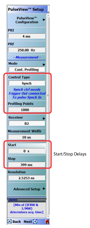
The PulseView menu for CProf only differs slightly from that for CPIP (see Figure: Menu for CProf). There is the addition of start and stop delays to indicate the profiling time interval (just as in regular pulse profiling) and there is the addition of the field for Profiling Points. As discussed previously, this is the number of measurement windows within the time record that will be analyzed and is not correlated with the number of sweep points.

Traditional S-parameter calibrations are used less often with CProf since there are points in the time record that may not correspond to a particular sweep point and the exact locations may vary with electrically long devices (working with window positioning can help as with Profiling but it becomes more complicated here due to the sweep interaction). Normalizations and related processes are frequently employed.

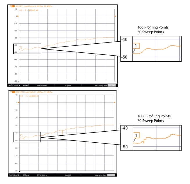
An example CProf measurement is shown in the top part of Figure: Example CProf Measurement with Same Number of Sweep Points but Different Numbers of Profiling Points with a relatively small number of profiling points (100 with 50 sweep points). The points generally pick out each sweep point with some duplication. The same sweep but with 1000 profiling points is shown in the bottom part of Fig. 23-42. Here the display is much more step-like since multiple measurement windows are processed while the hardware is at the same sweep point (the number of plotted display points is equal to the number of profiling points). There are also some drop-out points where the hardware is transitioning between sweep points. While more challenging to interpret, this allows one to study the interaction of DUT dynamics with the changing frequency or power of the sweep in detail.

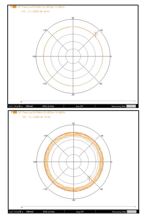
A slightly different kind of example is illustrated in Figure: Example CProf Measurement for Two Different Antenna Emulator Structures. Here a surrogate antenna pattern is being evaluated while frequency is sweeping. In the first case (an omni-directional emulator) has no frequency response over the interval. In the second case, the emulator has a high pass response so one sees a spiral formation in the ‘pattern’. This example helps show the flexibility possible with this measurement mode: the acquisition and analysis parameters are less constrained by the frequency/power sweep.