Standard Fast CW

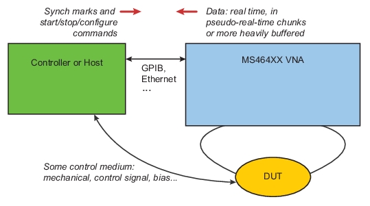
The standard Fast CW mode uses the basic instrument acquisition engine with the data paths simplified to increase speed and a number of additional commands introduced to control data flow and offer some configuration choices. The block diagram of the measurement is shown in Figure: Standard Fast CW Mode Measurement Configuration. The sources and receivers are programmed before the Fast CW process begins and triggering can be used to sequence between different Fast CW epochs (i.e., to move between frequencies, power levels, switch positions in the instrument, etc.). Once the Fast CW process begins, the measurement acquisition runs pretty much as fast as possible for a given bandwidth and either streams data out over the remote interface or dumps the data into an internal buffer for simplified access and handling. Synchronization within the data streams (which in some external literature is called ‘triggering’) is done with a data marking process that is similar in concept to that discussed in the pulse measurements chapter of this guide (PulseView™ (Option 35 and Option 42)). Conventional per-point triggering is permitted but will reduce the maximum speed to on the order of 10000 measurements/second. There is, however, a process for marking time within the data stream that will support the higher data rates which is discussed later in this section (a flag is placed in the data stream based on a separate command).

In this mode, data is made available as fast as possible over the remote interface with the speed usually limited by the remote interface itself. The ‘chunk’ size of data made available for transfer is adjustable from 1 to 500 measurements (with the definition of that term to be made clear shortly) to allow the user to optimize to their remote application in terms of transfer overhead, processing needs, etc. Although slightly unconventional, the data is shoved out onto the bus as fast as it is available and it is the responsibility of the user’s controller to grab the data (often with something like an fscanf command in C or various commercial control products) as it is available or samples may be missed. It is for this reason that the ‘chunk’ size is variable within a range. The size can be optimized for the practical speed and overhead requirements of the user’s interface.

This sub-mode is particularly useful when processing or control decisions have to be made in the middle of a measurement sequence. An example would be curtailment of a bias excursion once the DUT gain reached a certain level. Another example would be the halting of an antenna pattern measurement when the received power dropped below a certain level.

In this sub-mode, only one channel is used so all other channels are made inactive during the Fast CW measurement. Those channels will be restored and made active (if they were active before) when one exits the Fast CW mode. Most GPIB commands are blocked when in Fast CW because they interfere with the data transfer process (a detailed list is available in the programming manual) but a general rule is that all setup tasks should be performed prior to activating Fast CW and, if further setup changes are needed, one should exit Fast CW, make the changes, and then return.

There are two further types within the streaming sub-mode; Type 1: One response parameter and Type 2: Base unratioed parameters

In this case, the output is a single complex value representing the response parameter (which can be an S-parameter or a user-defined parameter) in the first active trace (‘active’ in the sense that it is turned on in Trace Management). In the preset setup (four traces: S11, S12, S21 and S22), S11 would be the parameter that is output. The response parameter is always transmitted to the remote interface in the form of a complex float in binary form so the transferred block would be of the form

#18<4 bytes for real><4 bytes for imaginary><EOL>

when a single measurement was requested. The format here is the standard binblock format discussed in the MS464XX Programming Manual (10410-00322):

If, for example, 3 measurements were selected for the ‘chunk’, then the data would come as the form

#224<4 bytes for real1><4 bytes for imaginary1><4 bytes for real2><4 bytes for imaginary2><4 bytes for real3><4 bytes for imaginary3><EOL>

In this case, the output consists of three complex values representing reference parameter for the current driving port (a1 or a2) and the two test parameters (b1 and b2). The current driving port is set by the first active trace (‘active’ in the sense of being turned on in trace management). The term ‘measurement’ in the earlier discussion still refers to one acquisition-set but now that is represented by three complex values. The parameters are always transmitted to the remote interface in the form of three complex floats in binary form so the transferred block would be of the form

#224<4 bytes for real_a><4 bytes for imaginary_a><4 bytes for real_b1><4 bytes for imaginary_b1 ><4 bytes for real_b2><4 bytes for imaginary_b2 ><EOL>

when a single ‘measurement’ was requested. The format here is the standard binblock format discussed in the MS464XX Programming Manual (10410-00322):

If, for example, 2 ‘measurements’ were selected, then the data would come as the form

#248<4 bytes for real_a_1><4 bytes for imaginary_a_1><4 bytes for real_b1_1><4 bytes for imaginary_b1_1 ><4 bytes for real_b2_1><4 bytes for imaginary_b2_1><4 bytes for real_a_2><4 bytes for imaginary_a_2><4 bytes for real_b1_2><4 bytes for imaginary_b1_2 ><4 bytes for real_b2_2><4 bytes for imaginary_b2_2><EOL>

In the 4-port case, if ports 1 or 2 are driving, a1=a2 will be provided (shared reference coupler). If ports 3 or 4 are driving, a3=a4 will be provided.

More details are available in the programming manual, but here is a synopsis of commands relevant to the streaming sub-mode.

Standard Fast CW Mode Measurement Configuration

The basic measurement configuration of the standard Fast CW mode is shown here. This is a remote-only mode and allows streaming or buffered data delivery.

Turns on the streaming Fast CW mode on the selected channel (ON or OFF).
Note that there is some delay between turning the mode ON and actual collection to allow for buffers to be set up. This can be as long as 100 ms.

Returns the state of streaming Fast CW mode on the selected channel.

Sets whether Fast CW will return the S-parameter data (SPAR), or the receiver data (RCVR). These correspond to type 1 and type 2 sub-modes discussed above, respectively.

Returns the current Fast CW mode

Outputs the data collected thus far in the form set by the current mode. Note that fscanf can be used for a no-command version of data retrieval in the streaming sub-mode.

Inserts a marker in the collected data. This is discussed more in the next sub-section. The command includes a 32 bit number that will be placed in the real field of the data (and the imaginary field will be set to 0) as soon as latency allows.

Sets the selected no. of points for streaming mode of FastCW in the given channel.

Outputs the selected no. of points for streaming mode of FastCW in the given channel.

Sets the type of collection. Choices are STREAM (for this section), HOLD, CONT, and STOP (HOLD and CONT are for the buffered sub-mode, STOP halts all collection and releases the buffers.

Outputs the current type of collection for Fast CW.

The buffered sub-mode is a bit different in that all of the data will flow into a potentially sizable memory buffer and the user can request data from that buffer when convenient or when the data is ready. The user can specify the size of the buffer and, when the data reaches that point, collection will cease and the CFB bit of the extended status register will be set (that can be polled by a remote application and there is a wait-based command WFFB which works like the WFS (wait for sweep) command used for regular T/R measurements). The query command :CALCulate:FCW:IBUF:POINts? can also be used to determine how many measurements are currently in the buffer (and the two types discussed under ‘streaming’ apply here as well so a ‘measurement’ can be 8 bytes (one parameter) or 24 bytes (3 unratioed parameters)).

The maximum size of the buffer is set by available memory which is constrained by the VectorStar application, the operating system and any other applications that may be running. The maximum is ~60 million points for type 1 (8 bytes per point) or ~20 million points for type 2. If other applications are running on the instrument’s PC or the PC memory is otherwise occupied, the effective maximum numbers may be reduced. The query command :CALCulate:FCW:MPCount? can be used to find the maximum allowable number of points at a given instant in time (but note the Fast CW must be ON for this command to produce an accurate value; a default maximum value will be provided otherwise). Note that the amount of time that this number of points represents is determined by the acquisition time per sample which is set by IFBW and point-by-point averaging. The minimum amount of time per sample (1 MHz IFBW and no averaging) is ~5 ?s.

While the data format is fixed (see the streaming section) for transmission over the remote interface, the user does have a choice of where in the post-processing chain the data is retrieved from.

The command is defined by

Sets the type of data to be collected in the internal buffer: Corrected, Final, or Raw.

Outputs the type of data that will be collected.

Some caution should be exercised with the last two choices in a very fast measurement scenario as the maximum speed can decrease and, if a 2-port calibration is involved, it can decrease dramatically as driving port switching is required).

One basic command controls the operation of the buffer.

This command sets whether the system should start collecting Fast CW data, stop collection, or pause (hold) collecting data (CONT, HOLD or STOP...the value STREAM is used for the streaming sub-mode).

Outputs the current data collection setting.

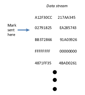
The command :CALCulate:FCW:MARK (sent as MARK x where x is a float (32 bit)) is used to mark the data stream. This is intended as a synchronization tool to indicate when the DUT is in a particular state (particular rotating antenna angle, different bias state, different switch state, etc.) without slowing down the process like a conventional triggering mechanism might. When the command is sent, the mark is inserted in the data stream as soon as possible (but it may take 20 μs or more for the mark to be inserted due to bus latencies) so it can be identified later. Any float can be used as the mark and, since data is stored and sent as real-imaginary parts, the mark is put in the real position while 0 is put in the imaginary position. Using 0 for the mark is often convenient as then a 0,0 pair will appear in the data stream and this is usually very easy to identify since an exact 0 almost never will occur in a live data stream due to the residual noise floor. An example of this process is shown schematically in Figure: MARK Marking Process in Data Stream when the mark value (in hex terms) was FFFFFFFF. Conceptually, the reader may notice similarities to External Sync Marking discussed in the Pulse measurements chapter of this guide (PulseView™ (Option 35 and Option 42)) and indeed they involve the same concept. The MARK process is not as direct since it must go through the remote interface layer so the latency is much higher than the ~5 ns for the sync marking process in Advanced Fast CW and in PulseView.

The MARK command also applies to the streaming sub-mode discussed earlier but, because of the more rapid transfers, the mark will be placed in the next available sub-chunk. The latencies are similar for the two sub-modes otherwise.

MARK Marking Process in Data Stream

The MARK marking process in the data stream (in hex form) is shown here. Part way into the stream, a mark with hex value FFFFFFFF was sent and placed in the real part of the next available point entry (the imaginary part of the mark is always set to 0).

As discussed earlier, there is some delay associated with turning on Fast CW (:CALC:FCW 1 or :CALC:FCW ON), particularly for the buffered sub-mode, as time is required to set up the buffers. This time can exceed 300 ms. To get a more accurate control of the timing (and allow for almost instantaneous MARKs at the beginning of the record), the following command sequence is suggested:

:CALC:FCW:DCOL HOLD (put the acquisition in hold while Fast CW is Off)

:CALC:FCW1 (Now turn on Fast CW)

…wait 300ms or more (give time for the buffers to be set up)

:CALC:FCW:DCOL CONT (now start acquisition with minimal latency)

Much as in the PulseView measurements chapter (PulseView™ (Option 35 and Option 42)), we use the term ‘triggering’ here to refer to an event to start a macroscopic measurement cycle. In the context of Fast CW, this usually means the initiation of the collection or the stopping and re-initiation of the collection (to change a frequency or power level for example). Thus, the external, GPIB and manual per-sweep trigger events have no effect when collection is in process. When the Fast CW mode is stopped, any of the above triggering modes can be used to re-initiate collection once the Fast CW process is armed. Per-point triggering is permitted but since the speed of the triggering interface in CW mode is limited to about 10 kHz, this will significantly limit the maximum data rates. Again, the MARK command is used to indicate events on a finer time scale within the collection period.

The acquisition speed in this mode is set by the IF bandwidth selection modified by point-by-point averaging with the maximum being with a 1 MHz IFBW and no averaging. The actual ADC-level acquisition rate in this case is ~1.5 MHz. Due to overhead in moving data around, the maximum rate that data can be put into the buffer (or otherwise made available) is approximately 200 kHz. This rate scales with decreases in IFBW or increases in averaging (roughly).


	Anritsu Company 1-800-ANRITSU 10450-00040 Rev. AB