The advanced CW measurement uses different IF and digital hardware internally that allows this mode to support much higher measurement rates and larger buffer sizes. The choice between these two modes may often be dictated by the rate-of-change of the system being tested. If changes of interest occur only on the scale of milliseconds, then the standard mode will probably be adequate. If changes occur on the scale a few microseconds or faster, the advanced fast CW method would be a likely choice. For intermediate cases, both modes can work and the choice may end of being one of synchronization flexibility, data handling details and convenience. The Advanced Fast CW mode does have a UI component so it does not need to be run remotely and there is a post-processing layer that can be used to isolate data of likely interest.

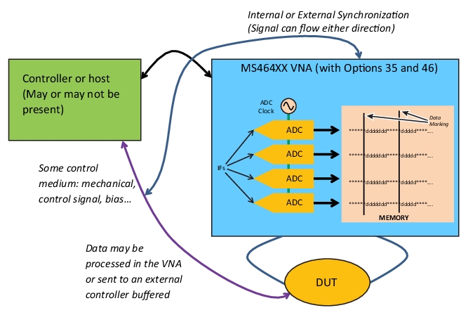
The measurement scheme is shown in Figure: Advanced Fast CW Acquisition Plan and the process is very similar, on a conceptual level, to a pulse profiling measurement discussed in PulseView™ (Option 35 and Option 42) (only without the pulses). When the measurement starts (which can be externally triggered), the data starts flowing into the digitizer memory. Periodic (or pseudo-periodic) marks can be placed in the data using an internal time reference or using external sync marking. Much as with the marking discussion in the previous section, this can be used to highlight a state-change on the DUT or the mechanical position of some part of the system under test (among other things). The latency of these marks is under 5 ns so the timing can be fairly precise. When internal sync is used, the marks are placed at a precise time interval specified by the user. When external sync is used, the marks are placed when a rising edge is sent to the Ext Synch In port on the instrument’s rear panel. The estimated period of sync marks should be entered (in the UI or remotely) when using external sync marking in order to simplify the plotting of data versus time but this is not required.

Some examples of different portions of the data that may be of interest:

Many of these types of data reduction are available from the instrument and the results plotted (and, of course, are also available remotely). In all of these analysis types, the entered IF Bandwidth and Point-by-point averaging values are not used. ‘Measurement width’ (which will be defined) controls effective bandwidth and sweep-by-sweep averaging can be used for trace noise reduction on a longer time scale.

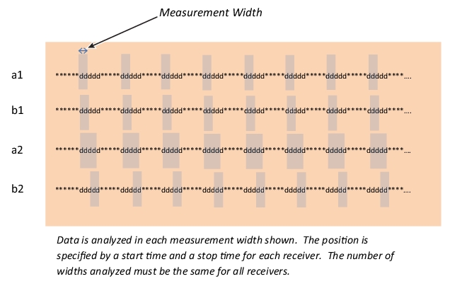
The simplest post processing to discuss is ‘full time record’ where samples can be analyzed with almost any density over the full set of data that was acquired. The concept of the ‘measurement width’, which may be familiar to readers of the pulse measurements chapter, is important. The user can specify how large a window should be analyzed to create a ‘point’ and this window width is expressed in terms of time. That amount of data in the time record will be blocked off and something similar to a discrete Fourier transform applied to create a ‘point’ with an effective bandwidth of 1/(measurement width). The available values depend on the acquisition rate (1/sampling interval) but for the default high speed rate, the minimum measurement width is 5 ns and the maximum is the depth of memory collected. The user also specifies a time range in total to be analyzed and how many points to be computed. The relationship of these variables is shown pictorially in Figure: Advanced Fast CW Processing Scheme—Full Time Record Sub-mode. Note that the widths and delays can be independently selected for each receiver. If a large number of points with a large measurement width are selected, the processing time will increase beyond seconds. In this method, the synchronization marks are not used except to denote the start of the measurement and, in this way, can function as a secondary triggering path that is much more closely tied to acquisition timing than is traditional external/GPIB/manual triggering so latencies are much lower and more predictable.

The full time record approach can be useful when transient behavior of the DUT is of interest (as it moves from one state to another for example) or when an analog variable is being changed (such as bias or mechanical angle of a receiving antenna) and there is a less discrete sense to the measurement.

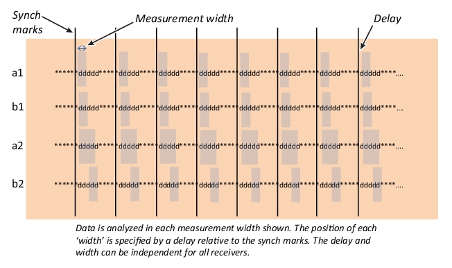
The other processing approach is point-by-point and is similar, in a calculation sense, to the pulse-to-pulse method in pulse measurements. The synchronization marks (whether they are internal or external) are central to this method since each analysis ‘point’ is associated with a mark. Much like the ‘full time record’ method, the measurement width defines the individual chunk of data to be analyzed but now the location of that chunk is defined by a time delay relative to the synchronization mark instead of in terms of absolute time. This processing approach is illustrated in Figure: The processing scheme for the ‘point-by-point’ sub-mode is shown here. and this method is useful when the various DUT states have a discrete nature to them and synchronization is possible (in either direction). It can also be used with no synchronization in which case the interval timing set on the instrument becomes the source of the timing marks.

Unlike in PulseView measurements, the concept of averaging between intervals does not apply so the IF bandwidth and point-by-point averaging values are not used. The measurement width controls the effective DFT bandwidth and the noise floor and trace noise. Sweep-by-sweep averaging is still available as this involves multiple acquisitions that can be combined and can, in particular, reduce trace noise. Note that there can be some triggering complications when using sweep-by-sweep averaging depending on the measurement since the DUT state will have to repeat on the multiple sweeps used.

Of course, the raw data (samples in time domain) can also be dumped for off-line processing. Because of the potential size of this data, it can only be saved in a binary format. To allow transportability, the format saves data into a sequence of 16 MB files. A MATLAB script for accessing the data is below and an executable version with some plotting and processing capabilities is available from Anritsu.

The format of the file names is

Ch1_fastcw_nnn.dat

Where nnn is an index number (first file is always 0, second file is generally 2097152, etc.). The file name preamble changes for different channels. For the code above and for the executables provided by Anritsu, it is important to not modify the file names or, if needed, to only add characters at the beginning of the file name (even then, the variable sA1 in the above code will need to be generalized).

An important point about the data is that each receiver has a field consisting of 14 data bits, one overrange bit and one synch bit forming 2 bytes per receiver. Data from all four receivers are always saved. The synch bit is common to all receivers as those paths are locked but the bit is repeated in the 2-byte-field for each receiver for convenience.

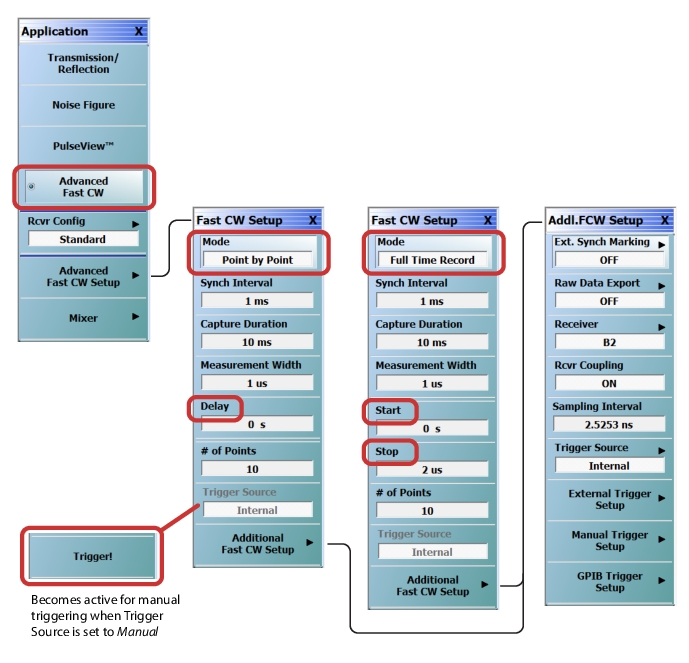
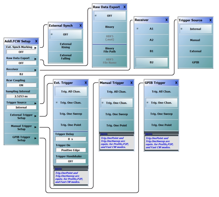
The parameters are all configured on the Advanced Fast CW setup menus shown in Figure: Advanced Fast CW Application Menus and Figure: Additional Fast CW Setup Sub-menus. The Enable Raw Data Save button brings up a file save dialog for the formats just described above. The Sampling Interval (equivalent to ‘Resolution’ in PulseView) and Capture Duration entries are analogous to concepts in PulseView and are described in more detail shortly.

Most of the remaining parameters have already been discussed as they configure the data analysis for the full time record and point-by-point subtypes. The Synch Interval relates to the synchronization marking interval (which could be internal or external as discussed) and is akin to Pulse Repetition Interval in PulseView. In the internal synch mode, this Synch Interval value is explicitly used for the time between synch marks. In external synch mode, it is the external signal that establishes the mark timing but the entry in the menu is used to help with labeling the x-axes on plots and for creating the independent variable vector for text-based data saving. The External Synch selection has three choices: Off (which implies internal synch), Ext. rising (external synch based on the rising edge) and Ext. falling (external synch based on the falling edge).

Note that the Trigger menu items have been replicated under the Fast CW menu for convenience. Changes made here will appear under the Trigger menu and vice-versa (they are the same control variables).

The Sampling Interval (1/ (acquisition rate)) is variable and this affects how much data in terms of time can be stored. At the default Sampling Interval near 2.5ns, the maximum depth is 0.5 seconds without the expanded memory option (Option 36) and 2.5 seconds with Option 36. The Sampling Interval can be increased to a maximum of 70 ns which leads to a maximum depth of 14 seconds or 70 seconds (without or with Option 36, respectively). In terms of useful data points that can be stored, the Sampling Interval does not matter but how the data is analyzed will have an impact on the maximum point count (here ‘point’ refers to a realized frequency domain measurement value). Since the raw time domain waveform is at the system IF, normally data is analyzed in terms of a short-time DFT as discussed earlier in this chapter and the classical minimum would be four time samples to form a data point. Under that rule, the maximum point count is 50 million or 200 million (without or with Option 36) for EACH of the four receiver channels (a1, a2, b1 and b2). Internally, fitting options are available that allow analysis on 2 or 3 time samples which allows the point count to increase to 100 million/400 million with a corresponding increase in trace/data noise. The time-shifting single sample approach that allows 2.5 ns resolution/Sampling Interval in the PulseView mode is not available in Fast CW due to slightly different data handling procedures. Of course, if larger amounts of effective averaging (more samples in the DFT), then the number of available ‘points’ will correspondingly decrease unless one starts to overlap time intervals. The latter is allowed (and can always be done offline) but introduces an effective smoothing function so that the time-resolution-of-data is not increasing as much as the point count would indicate.

Capture Duration (also termed Acquisition Length) has also been discussed in PulseView™ (Option 35 and Option 42) and simply informs the system how much data to collect in the buffer in terms of time. As listed in the previous paragraph, the maximum allowed value in this field is a function of the Sampling Interval. Note that the number of plotted frequency domain points in ‘point-by-point’ mode is capped at ~Capture Duration/Synch Interval since that ratio determines how many sync events can be stored (it may be one less depending on the delay value). In Full Time Record more, the Stop Time must be less than the Capture Duration.

Much as in the PulseView measurements chapter (PulseView™ (Option 35 and Option 42)), we use the term ‘triggering’ here to refer to an event to start a macroscopic measurement cycle. In the context of Fast CW, this means the initiation of the collection or the stopping and re-initiation of the collection (to change a frequency or power level for example). Thus, the external, GPIB and certainly manual trigger events have no effect when collection is in process. Once an acquisition is complete, the above triggering modes can be used to start another one. The per-point and per-sweep variants have the same effect since it is a CW mode. Again, the external sync marking concept is used to indicate timing events on the finer time scale within the acquisition.