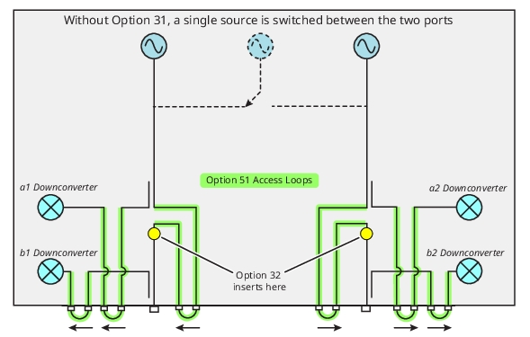
In some sense, Option 51 is the simplest of the RF options: it is to provide access to source and receiver paths. The isolated block diagram is shown in Figure: Option 51 and Access Loops. One important point is that the source loops are between reference and test couplers. For the labeling of the source loops, the base of the arrow corresponds to the source side and the pointed end corresponds to the side closer to the test port.
Option 51 and Access Loops
The block diagram showing the loops of Option 51 is presented here. Only front panel loops are shown in this figure which are for frequencies >=2.5 GHz. The loops for <2.5 GHz frequency access are on the rear panel. The arrows shown match the markings on the instrument.
Power leveling is done prior to the source loops so the ALC dynamics will not be affected by device added into the loop path but, of course, the power delivered to the port will be affected. User power calibrations are used to improve the accuracy of the power at the user reference plane and are particularly helpful when these source loop access points are used. An important point about the power calibrations when using a driver amplifier or other network in the source loops is the relationship between Entered power, Effective Power and Target Power (the former being on the top level of the Power menu and the last being entered as part of a user power calibration). Note that the leveling detection point is within the a1 and a2 coupling systems and hence precedes the source loop. For a leveling point that can include, for example, a pre-amplifier in the source loop, see Option 53 (external ALC) discussed later in Option 53/8x and External ALC Access.
Entered Power: This is the ALC system setting. When no user power calibration is applied, the system uses the factory ALC calibration to setup the hardware to provide close to the indicated value to the test port. When a user power calibration is applied, the power delivered may now be only loosely related to the ALC entry value.
Target Power: This is the value that the user power calibration will attempt to achieve. If a value here is unrealistic based on the instrument power range, devices added to the source loop, and networks between the instrument port and the reference plane, the calibration will fail or produce a large error.
Effective Power: This is a calculated value of the power available at the reference plane based on knowledge of the user power calibration and step attenuator settings (see Option 61/62). Immediately after a user power calibration, assuming it was successful, the Target Power will be available at the reference plane and the Effective Power will match the target power. If the Entered Power is changed after the user power calibration, the Effective Power will change by an equivalent amount.
Example:
The power menu Entered Power (ALC setting) is -10 dBm.
A user power calibration is to be performed with a Target Power of –15 dBm (which will be achievable unless ~>15 dB of gain or > 15 dB of loss (depending on frequency and instrument model) has been added to the source loop path or between the port and the reference plane).
After the calibration is complete, the Effective Power will read –15 dBm.
If the Entered Power on the power menu is now changed from -10 to –7 dBm, the Effective Power will change to –12 dBm. At the reference plane, approximately –12 dBm of power will be available (unless considerable loss has been added either to the source loop or between the port and the reference plane).
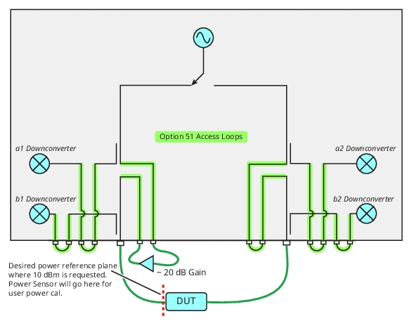
When a large gain or loss is added, more careful consideration of the Entered and Target power may be warranted. Consider the example of Figure: User Power Calibration Example where a relatively high gain amplifier has been added to the source loop (~20 dB) and a target power of 10 dBm is desired and the frequency range is 20 GHz to 30 GHz.
User Power Calibration Example
An example is illustrated here of performing a user power calibration with a relatively high gain amplifier added to a source loop.
If one used 10 dBm for the Entered Power and the Target Power, there may be unleveled messages displayed prior to the calibration (depending on the instrument model) and the driver amplifier will be initially exposed to power levels in that +10 dBm range. Not only may this be an issue for the amplifier, but it may also damage the power sensor that will be connected at the reference plane and it may hamper the ability of the calibration to complete (even if the sensor was not damaged) due to convergence issues. A reasonable practice is to deduct the gain from the Entered Power first (so –10 dBm would be entered). This need not be precise. It is only telling the system where it should approximately start the power search.
The source loops are labeled as having a damage limit of +20 dBm and this is somewhat conservative but pertains mainly to the loop side closer to the front panel (pointed end of the arrow).
The access loops for the receivers are positioned between the coupled arms of the couplers and the actual downconverters. One can directly access the receivers here for 13 dB to 20 dB higher sensitivity but a correspondingly lower compression point. Note the maximum power levels posted on the instrument; these primarily apply to the receiver inputs (the pointed end of the arrows). Amplifiers or pads can also be inserted into these loops to bias the receiver response towards lower or higher expected signal levels, respectively. Again, the noise floor (in port-referred dBm terms) and the compression point will move accordingly as networks are added here. Generally the 0.1 dB compression point at these receiver inputs will be at least 0 dBm.