Both lowpass and bandpass work similarly with regards to gating. Gating is the process of selecting or deleting certain defects to study. This can be left in time domain but, more commonly, the gated results are fed back through the forward transform to get the frequency domain result corresponding to the modified defect scenario just created.
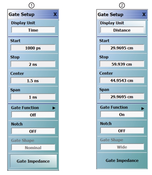
Gate Setup Menu
The Gate menu looks much like the Range Menu. The Display Unit toggle button and Start, Stop, Center, and Span buttons (for the gate this time) control values as described in the sections above.
The Notch toggle selects the polarity of the gate. When notch is OFF, the gate will keep everything between start and stop. When notch is ON, the gate will reject everything between start and stop.
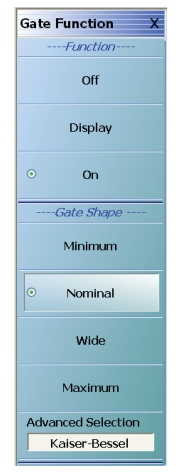
The default gate shape is nominal. By default, the gate is off. Selecting Display will allow the gate function to be drawn on screen (using the current graph type for the active trace). This can be helpful in visualizing what is being included in the gate. Turning gate on will apply the gate to the current time domain data.
The gate shape is analogous to the window selection. If the data was truncated with a sharp gate (minimum, akin to rectangular), maximum resolution is used determining the gate but ripple is introduced in the frequency domain. For more gradual gates, the resolution in separating defects decreases, but the size of the artifacts added to the frequency domain data decreases as well.
The window and gate shapes cannot be selected entirely independently since they interact through the transform. In particular, the use of a very sharp gate with a low side lobe window can lead to large errors. The allowed combinations are shown in Table: Window Type and Gate Shape—Allowed Combinations below. If an invalid combination is selected, the variable not being currently modified will be changed to the nearest valid value.
Window Type and Gate Shape—Allowed Combinations
Window/Gate
Minimum
Nominal
Wide
Maximum
Rectangular
OK
OK
OK
OK
Nominal
OK
OK
OK
OK
Low side lobe
No
OK
OK
OK
Minimum side lobe
No
No
OK
OK
With the advanced gates and windows, selections are not precluded although substantial errors can result if values are chosen without caution. If a more aggressive window is chosen (larger beta or side-lobe level), then the gate must be wider (wide or maximum; larger beta or side-lobe level).
DUT Example—Gate and Window Nominal
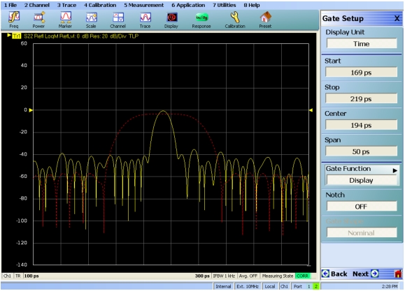
To work through an example, a DUT consisting of a short at the end of a slightly mismatched transmission line is used. It is desired to examine the short more closely in frequency domain, excluding the effects of the transmission line. In Figure: Gate in Display Mode Example, the gate is in display mode surrounding the desired reflection. Both gate and window are set to nominal in this case.
Gate in Display Mode Example
Gate is the red dashed line
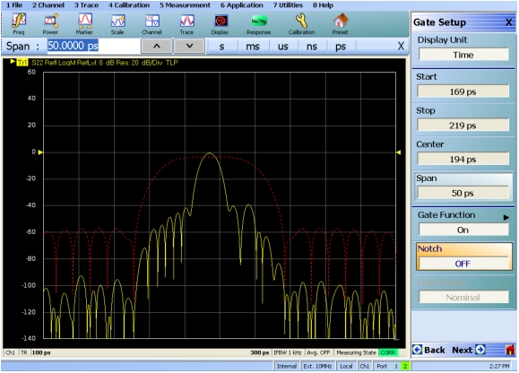
Next the gate is turned to on. In Figure: Gate Turned On Example, the suppression of the time domain information outside of the gate area is seen.
Gate Turned On Example
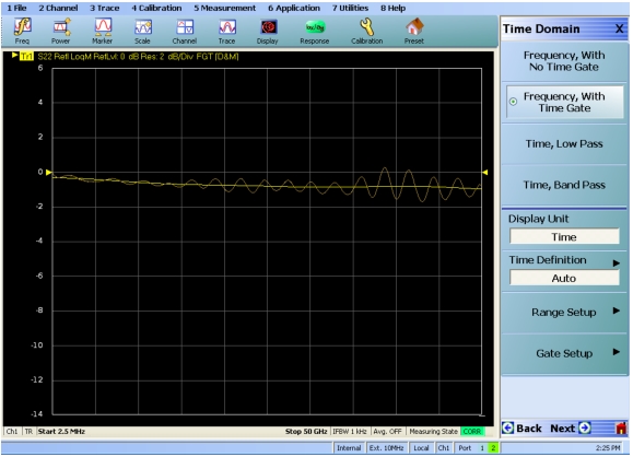
Finally, frequency with time gating is activated and the result is shown in Figure: Frequency with Time Gating Example. The result from frequency without time gating is shown in memory as a darker trace. The time gating has removed much of the ripple due to the mismatched transmission line and residual source match of the instrument.
Frequency with Time Gating Example
Other Frequency-with-time-gate Calculation Items
Questions are sometimes asked about the details of the gating process and the subject of uncertainty in the final result. The latter topic is addressed in the next section. In terms of the process itself, the basic concept is simple enough: a particular functional form (to exclude or include certain portions) is applied to the time domain data before it is returned to the frequency domain. As the time domain data is theoretically of infinite extent, the limited data roster forces some truncation to happen by default so even with an infinitely wide gate, the process is not conservative.
To get around this problem, a calibration signal (a single, synthetic tone) is applied to the current window/gate setup to generate a set of correction factors. Normally this does not introduce any significant errors. If the gate is very narrow (in the sense of approaching 1/BW), there is an additional issue in that the equivalent frequency domain convolution starts trying to interact more with frequencies outside of the sweep range. In the extreme case, this results in distorted final result, particularly at the extreme frequencies. To improve these results, the gate processing is done on a synthetically larger frequency range (using modeled extrapolation) to minimize out-of-range convolution effects. It is still advisable that the gate not be any narrower than a few resolution intervals.
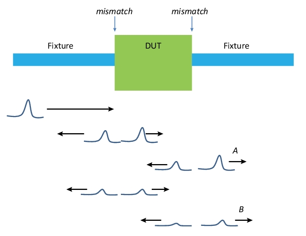
A second type of question that often arises is on how to use and interpret FGT results on transmission parameters. Suppose one had a device in a fixture, one might think that one could de-embed transmission by simply placing a gate around the appropriate place. Unfortunately, it is not quite that simple. Consider the time domain representation of an impulse traveling through our fixture + DUT assembly.
In the time domain sense, an impulse is incident from the left and, at the first interface, some is reflected and some is transmitted. The transmitted impulse then sees the output plane of the DUT and again, some is reflected and some is transmitted. The transmitted impulse (labeled ‘A’ in Figure: Illustration of Gating Effect on Pulse Re-reflections) goes to the receiver and this is the first response observed in the time domain transmission measurement.
Illustration of Gating Effect on Pulse Re-reflections
If one follows the remaining pulse energy, there is an internally reflected impulse in the DUT that again emerges towards the receiver (labeled B). There may be additional re-reflections that contribute depending on the loss and reflection levels. Now if one places a gate around ‘A’, one will remove the contribution of re-reflections and this may reduce the ripple in the FGT response. This is not complete de-embedding, however, since ‘A’ includes loss effects of the fixture as well as any incident mismatch—those effects were not removed by this gating process. For that fuller level of correction, more traditional de-embedding steps usually need to be followed.
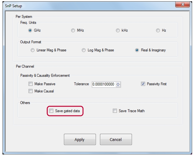
Saving of gated data into sNp files is enabled with a check on the SnP Setup dialog.
As might be expected, there is some potential for confusion on which gate is applied to which parameter. The following rules are employed:
• If gating is applied on no traces on the current channel, only ungated .sNp data will be saved.
• If gating is applied on at least one trace and the save gated field described above is checked, gated data will be saved for all parameters (that are part of the current .sNp save request). In this case:
• If all parameters of the .sNp are setup as gated in the current channel, those parameter-specific gate parameters will be used. The data from the last processed run will be used for the save.
• If not all parameters are setup as gated, the gate parameters of the first gated trace of the same parameter type (transmission/reflection) will be used. If such a trace does not exist, the gate parameters of the first gated trace will be used. If a trace does not exist for the required parameter, its measurement will be taken from the buffer (if a calibrated parameter) or a measurement re-triggered (if not a calibrated parameter but part of the sNp save definition).
• If gating is applied to the .sNp file, a comment line (! GATING applied) will be added to the header of the file.
Time Gating and Reference Impedances
When a gate starts or stops in a region whose impedance is not the reference impedance (usually 50 ohms), there can be some complications in interpreting the Frequency-with-Time-Gate result. Consider the example of a Beatty line (a 50 ohm transmission line with a length of 25 ohm impedance in the middle) shown in Figure: Sketch of a Beatty Line Structure. It will be used to illustrate a problem with gated reference impedances.
Sketch of a Beatty Line Structure
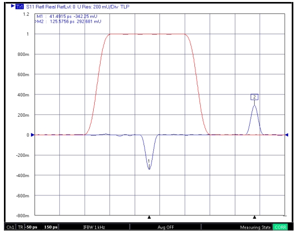
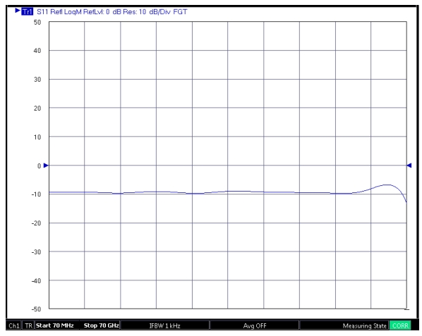
In impulse time domain (low pass in this case) with a gate in Display mode, the result for this example looks like that shown in Figure: Impulse Response of Beatty Line shown in Figure: Sketch of a Beatty Line Structure. At Marker 1, we reach the initial transition (50 ohms down to 25 ohms) so there is a negative going impulse. Suppose one wanted to gate and study the first half of the Beatty line back in the frequency domain. Since the gate will delete all further reflections, it is as if the line continued at 25 ohms forever and the FGT result like that shown in Figure: FGT Response for Gate Setup shown in Figure: Impulse Response of Beatty Line shown in Figure: Sketch of a Beatty Line Structure would occur (where there was some other parasitic structure present so the result is not completely flat). If one were to save a .s2p file of this result, this is essentially saying the reference impedance of the far port is 25 ohms. While this may be desirable in some cases, it is normally not what is expected by simulators or de-embedding engines and some additional action would normally have to be taken to get correct results. If referenced to 50 ohms, the result for S11 should have shown large peaks and valleys with spacing dependent on the length of the remaining 25 ohm section.
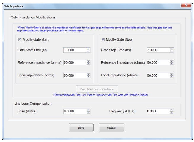
The Gate Impedance modification tool (accessed via Main | Display | Domain | Gate Setup menu | Gate Impedance | Gate Impedance dialog—see Figure: Gate Impedance Dialog) allows one to re-reference the impedance at either end of the gate to something that might be more desirable (often the calibration reference impedance which is usually 50 ohms). This process works by synthetically introducing impedance transitions at Gate Start and/or Gate Stop to get the net result back to the desired impedance planes. If, in the above example, one wanted to use the FGT result to create a de-embedding file for use in a 50 ohm system, then a modification only at Gate Stop would be required where the local impedance is 25 ohms.
Gate Impedance Dialog
Additional Notes:
• The system will calculate the local impedance at Gate Start and Gate Stop locations if requested. This calculation is based on a step response integration of the current data and can be helpful if the DUT impedance levels are not precisely known. Note that if the Gate Start or Gate Stop are placed very close (within a few impulse widths) to physical impedance transitions, the accuracy of this calculation will be reduced.
• If the DUT is lossy, the synthetic modifications should be based on that loss level as well as the impedances involved and the loss-per-unit length at a specific frequency can be entered. A square-root-of-frequency dependence will be assumed and the loss will be treated as being equally distributed along the length of the DUT (up until Gate Stop anyway).
• Local and reference impedances must be positive real.