As has been alluded to in the previous sections, many factors affect noise figure uncertainty and an understanding of their impacts and interactions can be important in setting up and performing a high accuracy noise figure measurement. The purpose of this subsection is to explore these effects and to produce a more realistic picture of the uncertainties one can expect and how to improve them.

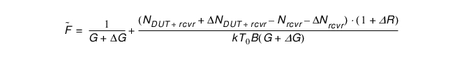
Looking back at the noise figure equation (Eq. 19‑4 above), one can recast it to show how component uncertainties affect the result. In Eq. 19‑6 above, the Δ terms represent deviations that may occur during the measurement or the calibration. Not all possible deviations are included here but rather only those that are most dominant practically are shown.

The Gain variance is perhaps the easiest to understand. Gain errors can arise in the usual s-parameter uncertainty context (or the equivalent for a frequency converting device) and this uncertainty is usually what is included. Errors due to linearity faults or other structural measurement problems are generally assumed to be taken care of by the user.

The other potential terms relate to the measurement of noise power and those are split into two groups: those common to both DUT measurement and calibration noise measurement (represented by ΔR) and those unique to the individual noise measurements (the two ΔN terms). All of these have several sub-terms.

These terms in turn have many dependencies on DUT S-parameters/gain, DUT noise figure, receiver noise floor, receiver linearity, source match, absolute signal levels, power sensor characteristics, etc. Because so many variables are involved, an uncertainty calculator has been created to help in analyzing some of the scenarios. A Monte Carlo approach is used since many of the variables have random distributions (particularly in phase) so a statistical analysis of the uncertainty may be more practically useful and is increasingly accepted as a preferred approach (e.g., [8]).

A few general observations can be made:

To understand the parameter space and to illustrate some of the computation options that are available, we will run through some examples.

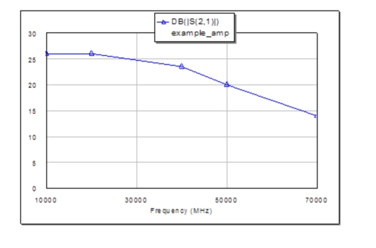
Consider an example amplifier with the following gain profile:

The DUT noise figure ranges from 3 dB at 10 GHz to 8 dB at 70 GHz with a frequency dependence that will be shown shortly. Consider the following example parameters:

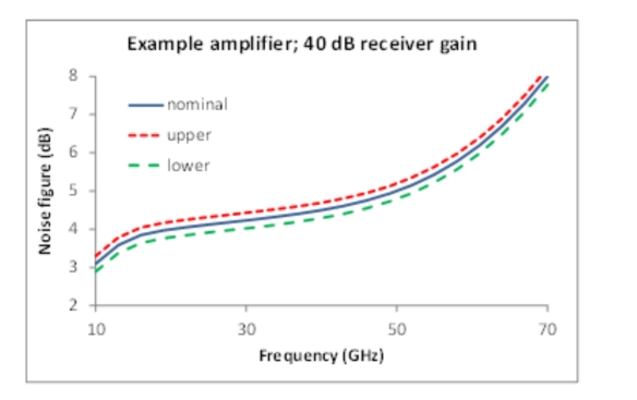
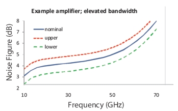
The first plot in Figure: Uncertainities for 40 dB Receiver Gain shows the nominal DUT noise figure (solid line) and the upper and lower 95% uncertainty bounds if the receiver gain is 40 dB.

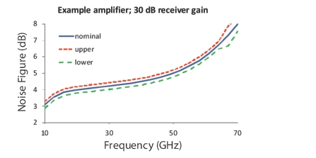
Next the receiver gain is reduced. Note that there is little change except at the higher frequencies where the DUT gain is low. This is a general concept that the DUT gain + receiver gain is a normative parameter.

Next, let us return the receiver gain to 40 dB but increase the measurement bandwidth to 30 kHz. This increases the data jitter and the net uncertainty.

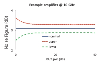
We can also look at a different independent variable. In Figure: Uncertainty as a Function of DUT Gain Plot, the receiver gain and IF Bandwidth have been returned to their starting values but we will plot versus DUT gain for a single frequency (10 GHz). As might have been surmised from the Figure: Behavior of |S21| with Example Amplifier discussion, if the gain gets low enough (in concert with receiver gain), the uncertainty will increase.

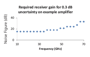
Finally, one may want to know the receiver gain for a given level of uncertainty. This is plotted in Figure: Required Receiver Gain Plot for our example amplifier (using nominal parameters) but with a 0.3 dB desired uncertainty. There is a step-like quality to the plot since the possible receiver gains are parameterized in ~2 dB steps for simplicity. As might be expected, as the DUT gain drops at higher frequencies (and noise floors increase in the VNA slightly), additional receiver gain is needed to hold the uncertainty constant.