In recent years, numerous improvements have been made in noise figure measurements through better algorithmic understanding of the measurements (e.g., [1]-[6]), more sensitive receivers, and simpler methods of processing noise power measurements. This chapter describes one specific set of improvements, based on the cold source measurement technique and related error correction techniques to enhance the noise measurement accuracy.

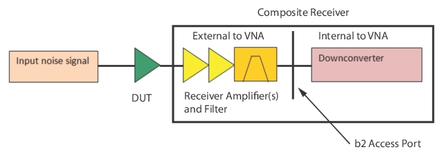
One particular avenue of noise figure measurements will be discussed here based on a cold source technique and some corrections applied to it. Before beginning with the algorithmic discussion, it may help to briefly look at the measurement hardware. In all cases, the DUT will feed a composite receiver consisting of the main receiver of the VNA augmented with amplification and filtering. The reasons for the extra gain will become clear later in this chapter. The basic structure of the VNA and DUT setup is shown below.

Historically, a popular method for noise figure measurements was termed a hot-cold or Y-factor technique in which a noise source was employed that could produce a low noise output power (cold = Nc) and an elevated one (hot = Nh). This noise source becomes the ‘Input Noise Signal’ in Figure: Noise Figure Measurement Basic Setup Diagram.

The ratio of measured noise powers in these two states was termed the Y-factor (Y = Nh/Nc) (e.g. [2]) and could lead to a quick calculation of noise figure (F) via the equation (Eq. 19‑1) below.

Where Th is the equivalent hot temperature of the noise source and the cold temperature was assumed equal to a temperature of 290 K = T0 (per IEEE definition).

By making a noise figure measurement of the receiver itself (Frcvr) and of the system (Fsys = FDUT + Receiver), it is possible to deconvolve the DUT noise figure with the familiar Friis’ equation (Eq. 19‑2) below: [1].

Here, the DUT gain G could be measured separately (via S-parameters) or it could be determined from the change in measured noise powers during calibration and measurement. One advantage of the hot-cold noise figure measurement method is that no absolute power calibrations are needed (all based on ratios). This was particularly important in the past when wide dynamic range power measurements over large bandwidths were more difficult. One challenge of this measurement method was the ability to provide a well calibrated noise source.

Because of the signal levels and bandwidths involved, accurate noise source calibration (for Th) is challenging and normally left to only a few metrology laboratories. In addition to issues in calibrating the noise source, a larger challenge occurred when the match of the noise source changed between the hot and cold states [4]. This could lead to large errors, particularly as the DUT input match worsened. These errors could be partially corrected using a source correction method (e.g., [3]).

The cold source noise figure measurement method was developed to eliminate the requirement for a multi-state noise source, which would the allow the use of a simpler, better controlled noise source (nominally a termination at room temperature). In this case, the noise figure is found from a simpler equation (Eq. 19‑3), but it has some subtleties:

Where:

To calculate the noise figure, there are a few key steps to accomplish.

First, an absolute noise power is now required (numerator N), so a means of a receiver power calibration is needed.

Second, an effective measurement bandwidth (B) is needed. Since measurement bandwidth is largely determined by the digital IF system, B can be pre-calculated. This bandwidth value may also be determined with the absolute power calibration step if a noise signal is used, otherwise it is determined separately.

Third, to isolate the noise figure of the DUT, the noise contributions of the receiver must be taken into account. As with the hot-cold method, a measurement of receiver noise is required with the cold source attached to the receiver input. Taking the receiver noise into account, Eq. 19‑3 above can be re-expressed in the form below (Eq. 19‑4):

A few things are immediately obvious: errors in gain or the noise power measurement will propagate to noise figure on roughly a dB-for-dB basis (if the gain is sufficiently high at least). These accuracies will be discussed throughout this chapter, but it is worth remembering the approximate dependence.

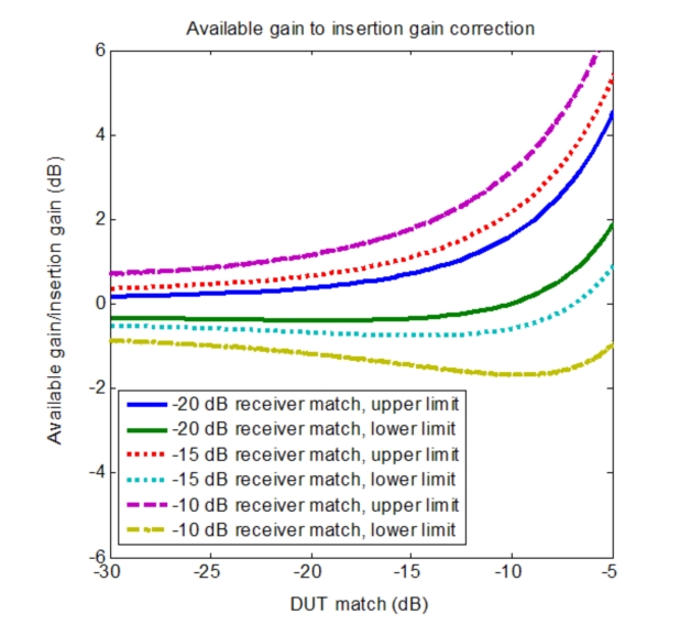
Of all of these terms, and it is true with hot-cold approaches as well, the term most often misvalued is the DUT gain. As has been discussed many times before (e.g., [3]), the noise figure definition is based on input noise power available to the DUT and output noise power available from the DUT. As a result, it is available gain that is the most appropriate value to use as opposed to insertion gain (which is what was commonly used with Y-factor approaches) or even |S21|2. As the DUT match worsens, the difference between these gain definitions increases. An example plot is shown in Figure: Differences Between Insertion and Available Gain as Function of Match Levels, where the DUT input and output matches (assumed symmetric for simplicity) form the x-axis and the receiver match is parameterized. The cold source match is assumed to be -20 dB and the DUT is assumed to have decent isolation (|S21 × S12|= 0.1). Multiple dB differences in gain, and hence in calculated DUT noise figure are possible as the match degrades beyond –10 dB.

In the case of the cold method (and assuming a quality termination is used on the input), it is primarily the DUT-receiver interaction that causes the difference in gain. From Eq. 19‑4, since gain errors map essentially linearly to noise figure errors, using the correct gain term is important even for commonly observed return losses.

Another potential source of errors in the noise figure measurement is the interaction of the receiver with DUT output. If the receiver noise power is strongly affected by the source impedance (i.e., a large Rn in the parlance of noise parameters), then significant errors could be encountered by not accounting for this interaction. This is accomplished by error correcting with the receiver noise parameters. To understand the relationship (e.g., [7]), recall that the noise response of a device (receiver in this case) may usually be characterized by four parameters sometimes represented by Fmin, Rn, and Γopt (which is complex hence counting as 2 parameters). Fmin is the minimum noise figure of the device when presented with an optimum source match (given by Γopt) and Rn is a sensitivity parameter describing the reaction of noise figure to changes in source match. The net noise figure of the device is given by (in this formalism) (Eq. 19‑5):

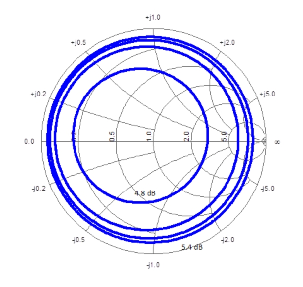
If Rn is small relative to the system impedance Z0, then the net noise figure is relatively insensitive to changes in the source reflection coefficient ΓS. Commonly, the effective receiver Rn is small and the dependency is minimal, since the receiver is normally a matched/feedback amplifier with some loss in front of it from cables, switching, and similar parameters. The noise circles of an example, typical receiver structure are shown below at 50 GHz. Even if the DUT output is very poorly matched (|S22|> –1 dB), the effective receiver noise figure only changes by ≈ 0.65 dB from Fmin. Assuming the DUT has ≈ 10 dB of gain and ≈ 2 dB noise figure; this would only add 0.1 dB of uncertainty. If the DUT had ≈ 20 dB of gain and ≈ 2 dB noise figure, this would only add 0.01 dB of uncertainty. With many common receivers, even less sensitivity is displayed although the effect is, of course, a function of which pre-amplifiers are used with that receiver.

If further reduction in uncertainty is desirable, it is relatively straightforward to add additional correction by including three additional measurements during the receiver noise calibration step (e.g., [4]). They are measuring the noise power with three reflect standards in addition to the cold noise source. Here one is just drawing on the long history of noise parameter measurement to help with an increase in receiver correction.

Another aspect of this measurement that sometimes receives less attention is that of linearity. Since it is a measurement of noise, a common perception is that there could never be anything nonlinear about the measurement process. Several issues do come into play

To illustrate the first point, suppose the receiver is composed of a 40 dB gain, 20 GHz broadband amplifier (plus some other components) before the downconverter and suppose the DUT also had about 40 dB gain and about 20 GHz of bandwidth. The input termination (cold noise source) will produce about –174 dBm/Hz noise power at room temperature. The integrated power at the output of the receiver amplifier (integrated over the 20 GHz) could reach +9 dBm (–174 + 80 +103). If the receiver amplifier compressed before this point (or if the downconverter did), then errors would occur. In this particular case, filtering would likely be needed anyway for image rejection (described in sections below) so this may not happen. If compression appears to be a problem, then less gain in the receiver path could be used.

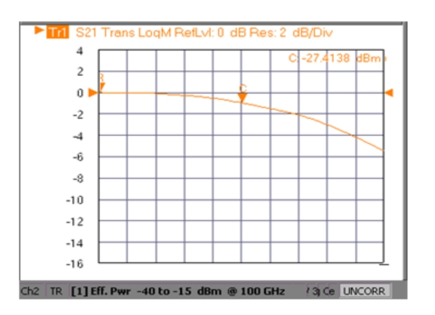
The second point is somewhat obvious, but one may not think to look at the DUT compression behavior if it is an LNA. The VNA default power ranges from –10 dBm to +5 dBm depending on model and options. This power range may not be appropriate for the DUT. By looking at |S21| of the DUT as power is varied or by using the gain compression tools in the power sweep modes (see Power Sweep (Swept Frequency)of this Measurement Guide for more information), one can ensure that the DUT gain data is obtained under linear conditions. As an example consider a W-band LNA whose noise figure was of interest. From the plot in Figure: Example of LNA Power Sweep, the DUT is already 1 dB compressed at an input power of ≈ –27.4 dBm at 100 GHz. The gain measurement in this case should be done at –35 dBm or lower.

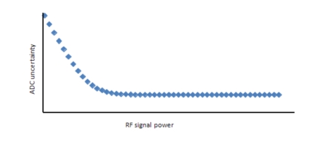
The third point, related to low level compression, is subtle but true for all analog-to-digital converters (used in every measuring receiver) at some point. In addition to quantization error, integral and differential non-linearities become most obvious at the lower signal levels that are implicit in a noise figure measurement (assuming one avoids the compression conditions described earlier!). In terms of sampling RF power, an ADC uncertainty plot may look something like the figure below. The plot suggests that there is a minimal level of receiver gain necessary to avoid problems from further down the IF chain of the system.

A key element in Eq. 19‑4 above, as yet unaddressed in this document, is the noise power itself. Historically, one way of measuring this quantity is a dedicated noise receiver with a large, variable gain system and appropriate filtering. This can be expensive and cumbersome and the typically wide bandwidths can lead to problems with narrowband devices (if the noise measurement bandwidth is close to the DUT bandwidth, including images, errors can result). Another approach is to use the basic VNA IF system itself, since it is highly linear to extremely low signal levels and has a fairly complete digital filtering system for tailoring the response shape. There may, however, be bias or leakage signal present in the response at these low levels that are not of interest. So in those cases, an RMS-like noise power measurement process is desired. In a non-ratioed channel measurement (usually b2/1), this net RMS noise power can be expressed as (Eq. 19‑6):

The reader may note the similarity to an equation for variance. Here N is a number of measurements (made at each frequency, termed a ‘number of RMS points’) and is typically a sizable number so that the effects of the mean (the second term in Eq. 19‑6) can be removed even if it is varying slightly with time. The default value of N is 3,000. Smaller numbers can be used for greater measurement speed (at the expense of some data jitter, more on this in the uncertainties section) and larger numbers can be used for some reduction in data jitter. Values of N greater than about 7,000 generally produce little benefit in data jitter reduction.

One may also ask how the unratioed parameter, |b2| in this case, comes to be a proxy for root-power. This comes via the receiver calibration (as is used for mixer, harmonic, IMD, and other measurements), since it transfers the traceable accuracy of the power sensor to the receiver parameter (|b2|). One may rely on the factory ALC calibration to provide the power reference for this calibration. It is more accurate to perform a user power calibration at the frequencies and level of interest prior to the receiver calibration to get the power accuracy roughly to the 0.1 dB level or better. Information on performing the power calibration is elsewhere in the measurement guide and operation manuals. When performing noise figure measurements, they are optimally performed at lower signal levels (e.g., –60 dBm using the internal step attenuators of Options 61/62 or an external attenuator) to stay in roughly the same part of the linearity curve as the noise figure measurement and to improve match. Performing power calibration at low signal levels (e.g. –60 dBm) may not always be practical. A low-level power measurement usually requires a diode-based power sensor, which are not readily available at frequencies above 50 GHz. At higher frequencies, a thermal sensor may be required for power calibration, which typically have a lower power measurement of ≈30 dBm.