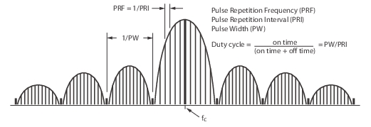
There are many methods of performing pulsed S-parameter measurements and each has different attributes. One method is based on the spectrum of a pulsed RF signal (shown in Figure: Narrowband Spectrum in Frequency Domain.) and capitalizes on the fact that the central spectral line carries the magnitude and phase information of the underlying RF signal.
After filtering everything but this line, standard VNA processing can be applied. The time separation for the measurement (receive-side) must be done in hardware (for example, a modulator would be used for profiling on the receive-side). This approach is known by several names, including band-limited, narrowband, and others. The central spectral line is filtered off and used in the band-limited or narrowband method.
This line spacing is set by the Pulse Repetition Frequency (PRF), while the sin(x)/x null spacing is set by the pulse width. For low duty cycles, progressively less energy is contained in the central spectral line, which results in dynamic range reduction.
From a processing point-of-view, this method is attractive because it only involves one frequency. However, it does suffer from some significant limitations:
• Since only the central spectral line is kept, energy is being discarded, particularly as the duty cycle of the receive pulse shrinks. The result is a dynamic range penalty of 20 * log10 (duty cycle). Using this method, when the duty cycle reaches 0.1 %, 60 dB of dynamic range has been lost.
• Calibrations must be repeated for every different pulse configuration. (The same is true to a certain degree for all methods. However, because of the above dependence of signal level on duty cycle, the effect is extremely strong when applying this method.)
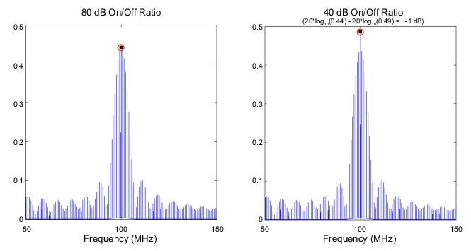
• The on/off ratios of the receive-side modulators can limit uncertainty. To illustrate the concept, consider the effect on the spectrum of imperfect isolation in a modulator between on and off states. When the pulse is supposedly off, there is information being retrieved that can be thought of as another pulse with a duty cycle equal to one minus the duty cycle of the main pulse.
The spectra will be centered at the same frequency (the IF) and the comb spacing will be the same, but the lobe structure will be different because of the different duty cycles. The result will be an interfering (different phase) central spectral line. The interference causes an increase in measurement uncertainty. As might be expected, the uncertainty impact gets worse for low duty cycles and poor on/off ratios.
• Receive-side modulation is needed on all parameters of interest. If full term correction is needed and the DUT exhibits notable intra-pulse behavior on the reflection parameters, then multiple test-side modulators are needed, even for an S21 measurement. Two source-side modulators would normally be required for full term corrections, unless pulse behavior in the reverse direction was not of interest or concern. The rise-time of those modulators and their associated bandwidths can limit resolution.
Narrowband Spectrum in Frequency Domain.
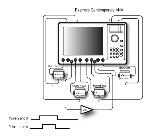
A setup for use in profiling applications is shown in Figure: Example Setup for Band-limited or Narrowband Profiling Measurements.. While an RF modulator is shown here on the receive side (receiver gating), an IF modulator could also be used. In this case, a minimum resolution limitation is incurred if the energy distribution is limited by the IF bandwidth.
In this setup, the receive-side modulator could be omitted if the average performance over the entire pulse is of interest (for example, in some cases where pulsing is done only to prevent the device from overheating and a conservative duty cycle is employed). The source-side modulator could be omitted if bias pulsing only is being used.
Example Setup for Band-limited or Narrowband Profiling Measurements.
Another method, termed a 'triggered' measurement, has been used mainly for slower repetition rate situations, where the VNA measurement is triggered to make classical measurements on sequential pulse (or synch pulse) rising edges. This method avoids the duty cycle dependence of the band-limited method and can allow for simpler profiling, if one has sufficiently precise control of the delay between trigger event and the actual measurement.
Trigger indeterminacy in contemporary VNAs is often large, resulting in a minimum pulse width that can be analyzed (often on a scale of tens or hundreds of microseconds). A second challenge lies in the data acquisition rate of many VNAs. VNAs have not traditionally incorporated precision high-speed digitizers, leading to poor timing resolution and inadequate profiling accuracy.
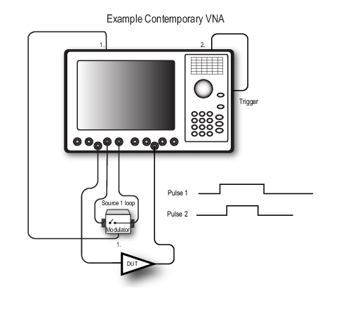
Calibrations often must be repeated for different parameter setups since the acquisition is being reconfigured. An example triggered measurement setup is shown in Figure: Typical Triggered Measurement Setup.
Receive-side modulators are normally not used in this scenario, except for certain (usually antenna-based) measurements, where leakage pulses can overwhelm the VNA receivers. This class of measurement will be discussed later.
Typical Triggered Measurement Setup
Historically, this setup has limited measurements to relatively low PRFs and wide pulses.
High-Speed Digitizer Measurements
A variation on the triggered measurement technique is the method implemented in the MS464xB Series VNAs. It is also based on direct acquisition, but at a much higher data rate. As a result, resolution is enhanced and time referencing is highly accurate. The exact acquisition method differs in that the acquisition is not controlled by the pulse system, but by the portions of the data record to be analyzed. The acquired data is then correlated with the pulse pattern being used.
Note
Pulse-to-pulse measurements are an exception to this method. This type of measurement is covered in Pulse-to-Pulse.
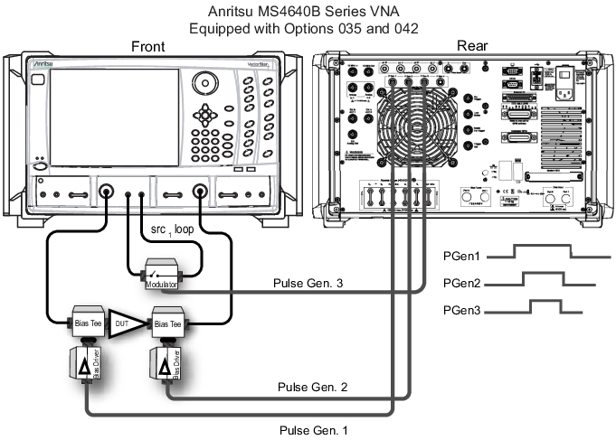
An example test setup is illustrated in Figure: Example Setup of the Fast Acquisition Method. Two bias supplies were used in this example along with stimulus pulsing. However, a different number of pulsed bias supplies could be used or stimulus pulsing could be removed. Receiver pulsing may be used as well.
The MS464xB Series VNA with Options 35 and 42 provides a four channel internal pulse generator and configuration software for driving bias pulsers, DUT control, and RF stimulus modulators (available in the pulse modulator test set) or RF receive-side modulators for special applications (in the four modulator versions of the test set; for more information on the pulse modulator test sets, refer to Setup Examples for Pulse Modulator Test Sets). An input/output of the T0 sync pulse is also provided so external pulse generators can be synchronized with the internal system (as might be needed in more complex bias situations).
No pulse generator channels are used to control the pulse measurement or profiling directly; this task is handled internally. The MS464xB Series VNA may be connected to an external trigger for pulse-to-pulse measurements and related measurements when the behavior relative to an absolute start time is important.
Example Setup of the Fast Acquisition Method
An example setup of the fast acquisition method of the MS464xB Series with Options 35 and 042. (Not all of the pulse connections shown must be used, and additional connections may be employed with this setup.)
Time records of the IF data are acquired at a high sampling rate, enabling the pulsed signals to be dissected into any of the desired pulse measurement modes. The resolution is on a nanosecond scale and the timing accuracy is very high without any duty cycle/dynamic range limitations on performance.
By using a fast digitizer and performing the alignment with pulse data in a post-processing sense, trigger latency issues associated with triggered measurements and potential jitter/inconsistency problems with that triggering are avoided. The resolution is set mainly by the acquisition rate instead, which is near 400 MHz. The jitter level is on the scale of picoseconds. When an external T0 synch is used, there may be an inconsistency on the scale of nanoseconds as the internal system must lock onto the external pulse.
Since no energy is being discarded in this setup, there is no duty-cycle dependence and the full dynamic range (>100 dB normally depending on IFBW, power levels and averaging) is available. Even for full correction, no receive-side modulators are required and the on/off ratio, bandwidth, rise-time and video limitations of those structures are no longer an issue. A deep memory (4 GB) is used to acquire long time records of up to one-half second. For sub-Hz repeat rates, the triggered method is an adequate choice as the jitter on that time scale will not normally be significant.
Pulse Measurement Terms and Synonyms
A number of other terms for pulse measurements are commonly used. This list will help to explain terms used elsewhere in this chapter.
Duty cycle or duty factor
Pulse width relative to the pulse period, often expressed as a percentage. Common values range from 0.01 % to 50 %. This may pertain to a stimulus RF pulse, a bias pulse, a receiver gating function, or a profiling pulse, so context matters.
PRI and PRF
Pulse repetition interval (= pulse period) and pulse repetition frequency (= pulse repetition rate). PRI=1/PRF.
Pulse width and delay
These two numbers together with the PRF uniquely define a pulse train; however, there are cases when there are multiple pulses per period (see below).
Note
The MS464xB Series always references delay to the rising edge of the T0 synch pulse, so that global timing can be easily defined.
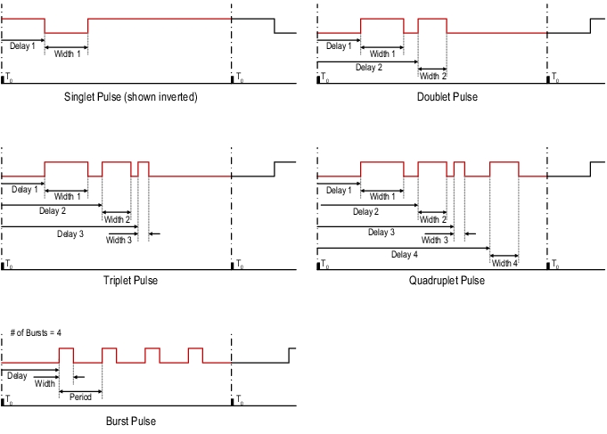
Defines what occurs once during each pulse period of the master clock. The default is a single pulse, hence the term 'singlet'. Sometimes more than one pulse is required per master clock period, hence other settings are available. “Burst” is a user-defined number of pulses within a period. All sub-pulse widths are the same and all intra-sub-pulse gaps are the same; see Figure: Timing Relationships for Multiple-pulses-per-PRI Signals. (Multiple pulses per period are particularly common in radar applications.)
Record length
The amount of time to be captured within a measurement. This is dependent on the PRI and duty cycle, the amount of averaging requested, and the measurement mode.
Synch pulse (T0)
This pulse establishes global timing and can either be generated by the MS464xB Series instrument or by an external pulse generator (in which case, the MS464xB Series can accept that signal as an input). For example, when coherence is needed among pulse generators, a common synch pulse is often shared between them. Synchronization of 10 MHz timebases may be needed as well.
Tstart and Tstop
These terms apply to pulse profiling setups and define the time range of interest relative to the synch pulse for profiling. Together with the number of time points, the measurement window width, and the requested averaging, these define the acquisition and processing behavior for pulse profiling. Tstart and Tstop can also be used as parameters for plotting data in pulse-to-pulse measurements.
Measurement width or Aperture
This measure of time describes what portion of the pulse should be analyzed in a given measurement. For point-in-pulse and pulse-to-pulse measurements, it is the section of the pulse to be processed (with a delay parameter specifying where, relative to T0, this window should be). For pulse profiling, this width is 'swept' across the pulse with processing across the measurement width being performed at each time step requested between Tstart and Tstop.
Timing Relationships for Multiple-pulses-per-PRI Signals
Measurement Modes
Pulse parameters and measurement definitions create an entire new parameter space to investigate. Many different terms have been used to describe these parameters in the literature; this document will try to conform to the most common usage. The terms will be defined in this section as used in the MS464xB Series.
Point-in-Pulse
This measurement quantifies S-parameter data somewhere within a pulse. One may want to avoid edge effects or just measure the pulse as a whole, but the structure within the pulse is not of great interest, nor is the variation from pulse to pulse.
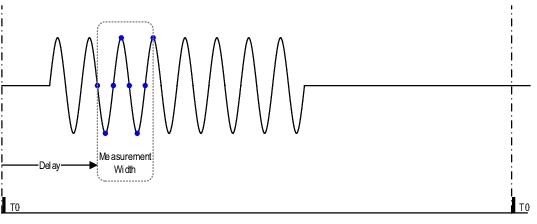
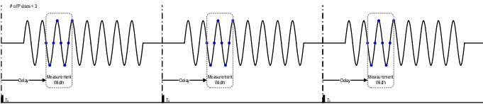
A point-in-pulse measurement is illustrated in Figure: Simplified Point-in-pulse Measurement Example. Data is acquired over a requisite length of time, and the user specifies the interval of interest relative to a sync pulse T0. This interval is usually quantified in terms of a delay and a desired measurement width or aperture. In addition, a level of averaging can be specified so this same interval is analyzed on multiple pulses and the results combined. Pulses are sampled with the same coherent clock so that phase information is maintained.
The diagram in Figure: Simplified Point-in-pulse Measurement Example illustrates an example where the width of interest is eight samples. While only a single sample is required for measurement, about four hundred million samples are possible (limited only by the record length of the instrument). Point-in-pulse measurements are often made with swept frequency or power, and are plotted as such. In these cases, the above process is simply repeated for multiple frequencies and power levels.
Simplified Point-in-pulse Measurement Example
Pulse Profiling
The pulse profiling measurement focusses on the structure of data within the pulse. Characteristics like overshoot or undershoot, droop, and edge response are measured, while the frequency and power are kept constant (although they can be varied between acquisitions).
This data is normally plotted vs. time to indicate position within the pulse (measurement normally is setup as constant frequency (CW) and constant power, but more complex measurements can be orchestrated using multiple channels or setups).
Variation between pulses is often not observable in this measurement, which may represent an average over a number of pulses. One can structure the measurement, however, to look at behavior from an absolute start time with no averaging in order to look at the complete evolution over multiple pulses.
A start time and a stop time (Tstart and Tstop) are specified relative to the synch pulse (T0) along with a number of time points to describe the portion of the pulse to be profiled. The measurement may begin before the physical pulse is at the DUT and end after the pulse is no longer being applied to the DUT, but the data must be interpreted appropriately in all cases. A measurement width is also specified (illustrated as eight samples in the diagram). Additional averaging can be imposed across multiple pulses, as discussed previously. As with point-in-pulse, the range of allowed widths is large.
The measurement windows are allowed to overlap (and will if (Tstop – Tstart) / (NumTimePoints – 1) < Width), which performs a variety of time-based smoothing operations on the data. A common setup is 10 to 20 non-overlapping (or slightly overlapping) profiling time points within a pulse, but application requirements may dictate very different parameter choices.
Example of Pulse Profile Measurement
Pulse-to-Pulse
Pulse-to-pulse measurements concentrate on variations between pulses that begin with an absolute start time. This type of measurement can be described as a hybrid of the first two methods. Normally one will pick a section of the pulse to measure, and then the progression over a number of pulses is plotted (versus time or index).
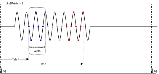
This process is illustrated in Figure: Simple Pulse-to-pulse Measurement., where the first three pulses are shown. The delay from T0 is the same for each measurement window of interest and the window in each pulse is processed separately.
Pulses are treated in an absolute fashion, so averaging of multiple pulses is not useful and is not available. As with pulse profiling, this measurement is performed at constant frequency (CW) and constant power. One could orchestrate measurements that cycled through a variety of frequencies and power levels using multiple channels or setups.
Simple Pulse-to-pulse Measurement.
A wide range of window widths (and pulse widths) is available as in the previous modes. The upper limit is set by the record length with options for very wide pulse or low rep repeat rates.
Note
The minimum measurement for the pulse-to-pulse measurement mode is two samples.
Important Measurement Considerations
Consider the bandwidth implications of all measurement methods in the sense of the smallest measurement window or profiling width that can retain device information without being overwhelmed by system effects before moving on with measurements.
Band-limited Measurement Modes
• In the case of the band-limited method, the system bandwidth limitations are derived from the receive-side modulator response shape, which forms a minimum resolvable pulse.
• If this modulation is done at RF (as has been suggested so far), then the rise/fall time of that modulator defines this limit.
• If the modulation is done at the IF, the same concept applies but only when the modulation is considered in the context of the IF system.
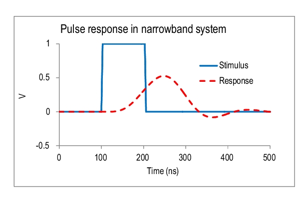
An example of these effects can be demonstrated when a DUT output pulse with 100ns width (3ns rise and fall time) is sent through an IF system with a 5 MHz bandwidth.
The pulse response is illustrated in Figure: Example Stimulus Pulse and Resultant Distorted Response Pulse. It is heavily distorted in this case, and a substantial ring-down is induced by this narrow IF system. The MS464xB equipped with Options 35 and 42 has a much wider equivalent IF and subsequent higher performance.
Example Stimulus Pulse and Resultant Distorted Response Pulse
Example stimulus pulse and resultant response pulse distorted by a finite IF bandwidth in a narrow bandwidth system.
Triggered Method
In the triggered method, resolution is generally limited by timing consistency of triggering and will be on a much longer time scale than either the band-limited techniques or the high‑speed digitizing techniques of the MS464xB Series equipped with Options 35 and 42.
High Speed Digitizer Method
In the high-speed digitizer pulse measurement method, there is generally no receive side modulator (except in the special cases). In its nominal operating state, this measurement method uses an IF of 100 MHz with appropriate filtering to avoid image responses.
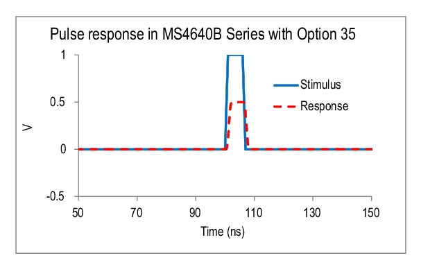
Artifacts include some edge softening, but the distortion is relatively small (especially when compared to narrowband systems; see Figure: Example Stimulus Pulse and Resultant Distorted Response Pulse). The amplitude was not scaled for this plot and the time shift is due to group delay in the system that must be accounted for in the measurement process.
Effect of the IF Bandwidth on the Pulse Shape
The effect of the IF bandwidth on the pulse shape using the MS464xB Series-035/042 measurement method and a 5ns wide DUT pulse with 1ns rise and fall times.
From these figures, we can conclude that a sufficiently wide IF, relative to the pulse shapes of interest, is important to ensure measurement of the DUT characteristics rather than those of the instrumentation.